Climate Experts Attacking a Journalist by Misinformation on Global Warming

Summary

Journalist David Rose was attacked for pointing out in a Daily Mail article that the strong El Nino event, that resulted in record temperatures, was reversing rapidly. He claimed record highs may be not down to human emissions. The Climate Feedback attack article claimed that the El Nino event did not affect the long-term human-caused trend. My analysis shows

  • CO2 levels have been rising at increasing rates since 1950.
  • In theory this should translate in warming at increasing rates. That is a non-linear warming rate.
  • HADCRUT4 temperature data shows warming stopped in 2002, only resuming with the El Nino event in 2015 and 2016.
  • At the central climate sensitivity estimate of doubling of CO2 leads to 3C of global warming, HADCRUT4 was already falling short of theoretical warming in 2000. This is without the impact of other greenhouse gases.
  • Putting a linear trend lines through the last 35 to 65 years of data will show very little impact of El Nino, but has a very large visual impact on the divergence between theoretical human-caused warming and the temperature data. It reduces the apparent impact of the divergence between theory and data, but does not eliminate it.

Claiming that the large El Nino does not affect long-term linear trends is correct. But a linear trend neither describes warming in theory or in the leading temperature set. To say, as experts in their field, that the long-term warming trend is even principally human-caused needs a lot of circumspection. This is lacking in the attack article.


Introduction

Journalist David Rose recently wrote a couple of articles in the Daily Mail on the plummeting global average temperatures.
The first on 26th November was under the headline

Stunning new data indicates El Nino drove record highs in global temperatures suggesting rise may not be down to man-made emissions

With the summary

• Global average temperatures over land have plummeted by more than 1C
• Comes amid mounting evidence run of record temperatures about to end
• The fall, revealed by Nasa satellites, has been caused by the end of El Nino

Rose’s second article used the Met Offices’ HADCRUT4 data set, whereas the first used satellite data. Rose was a little more circumspect when he said.

El Nino is not caused by greenhouse gases and has nothing to do with climate change. It is true that the massive 2015-16 El Nino – probably the strongest ever seen – took place against a steady warming trend, most of which scientists believe has been caused by human emissions.

But when El Nino was triggering new records earlier this year, some downplayed its effects. For example, the Met Office said it contributed ‘only a few hundredths of a degree’ to the record heat. The size of the current fall suggests that this minimised its impact.

There was a massive reaction to the first article, as discussed by Jaime Jessop at Cliscep. She particularly noted that earlier in the year there were articles on the dramatically higher temperature record of 2015, such as in a Guardian article in January.There was also a follow-up video conversation between David Rose and Dr David Whitehouse of the GWPF commenting on the reactions. One key feature of the reactions was claiming the contribution to global warming trend of the El Nino effect was just a few hundredths of a degree. I find particularly interesting the Climate Feedback article, as it emphasizes trend over short-run blips. Some examples

Zeke Hausfather, Research Scientist, Berkeley Earth:
In reality, 2014, 2015, and 2016 have been the three warmest years on record not just because of a large El Niño, but primarily because of a long-term warming trend driven by human emissions of greenhouse gases.

….
Kyle Armour, Assistant Professor, University of Washington:
It is well known that global temperature falls after receiving a temporary boost from El Niño. The author cherry-picks the slight cooling at the end of the current El Niño to suggest that the long-term global warming trend has ended. It has not.

…..
KEY TAKE-AWAYS
1.Recent record global surface temperatures are primarily the result of the long-term, human-caused warming trend. A smaller boost from El Niño conditions has helped set new records in 2015 and 2016.

…….

2. The article makes its case by relying only on cherry-picked data from specific datasets on short periods.

To understand what was said, I will try to take the broader perspective. That is to see whether the evidence points conclusively to a single long-term warming trend being primarily human caused. This will point to the real reason(or reasons) for downplaying the impact of an extreme El Nino event on record global average temperatures. There are a number of steps in this process.

Firstly to look at the data of rising CO2 levels. Secondly to relate that to predicted global average temperature rise, and then expected warming trends. Thirdly to compare those trends to global data trends using the actual estimates of HADCRUT4, taking note of the consequences of including other greenhouse gases. Fourthly to put the calculated trends in the context of the statements made above.


1. The recent data of rising CO2 levels
CO2 accounts for a significant majority of the alleged warming from increases in greenhouse gas levels. Since 1958 CO2 (when accurate measures started to be taken at Mauna Loa) levels have risen significantly. Whilst I could produce a simple graph either the CO2 level rising from 316 to 401 ppm in 2015, or the year-on-year increases CO2 rising from 0.8ppm in the 1960s to over 2ppm in in the last few years, Figure 1 is more illustrative.
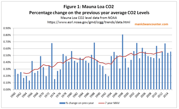
CO2 is not just rising, but the rate of rise has been increasing as well, from 0.25% a year in the 1960s to over 0.50% a year in the current century.


2. Rising CO2 should be causing accelerating temperature rises

The impact of CO2 on temperatures is not linear, but is believed to approximate to a fixed temperature rise for each doubling of CO2 levels. That means if CO2 levels were rising arithmetically, the impact on the rate of warming would fall over time. If CO2 levels were rising by the same percentage amount year-on-year, then the consequential rate of warming would be constant over time.  But figure 1 shows that percentage rise in CO2 has increased over the last two-thirds of a century.  The best way to evaluate the combination of CO2 increasing at an accelerating rate and a diminishing impact of each unit rise on warming is to crunch some numbers. The central estimate used by the IPCC is that a doubling of CO2 levels will result in an eventual rise of 3C in global average temperatures. Dana1981 at Skepticalscience used a formula that produces a rise of 2.967 for any doubling. After adjusting the formula, plugging the Mauna Loa annual average CO2 levels into values in produces Figure 2.
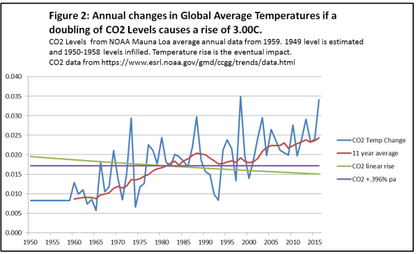
In computing the data I estimated the level of CO2 in 1949 (based roughly on CO2 estimates from Law Dome ice core data) and then assumed a linear increased through the 1950s. Another assumption was that the full impact of the CO2 rise on temperatures would take place in the year following that rise.

The annual CO2 induced temperature change is highly variable, corresponding to the fluctuations in annual CO2 rise. The 11 year average – placed at the end of the series to give an indication of the lagged impact that CO2 is supposed to have on temperatures – shows the acceleration in the expected rate of CO2-induced warming from the acceleration in rate of increase in CO2 levels. Most critically there is some acceleration in warming around the turn of the century.

I have also included the impact of linear trend (by simply dividing the total CO2 increase in the period by the number of years) along with a steady increase of .396% a year, producing a constant rate of temperature rise.

Figure 3 puts the calculations into the context of the current issue.
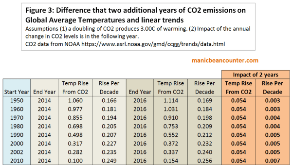
This gives the expected temperature linear temperature trends from various start dates up until 2014 and 2016, assuming a one year lag in the impact of changes in CO2 levels on temperatures. These are the same sort of linear trends that the climate experts used in criticizing David Rose. The difference in warming by more two years produces very little difference – about 0.054C of temperature rise, and an increase in trend of less than 0.01 C per decade. More importantly, the rate of temperature rise from CO2 alone should be accelerating.


3. HADCRUT4 warming

How does one compare this to the actual temperature data? A major issue is that there is a very indeterminate lag between the rise in CO2 levels and the rise in average temperature. Another issue is that CO2 is not the only greenhouse gas. More minor greenhouse gases may have different patterns if increases in the last few decades. However, the change the trends of the resultant warming, but only but the impact should be additional to the warming caused by CO2. That is, in the long term, CO2 warming should account for less than the total observed.
There is no need to do actual calculations of trends from the surface temperature data. The Skeptical Science website has a trend calculator, where one can just plug in the values. Figure 4 shows an example of the graph, which shows that the dataset currently ends in an El Nino peak.
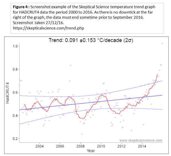
The trend results for HADCRUT4 are shown in Figure 5 for periods up to 2014 and 2016 and compared to the CO2 induced warming.
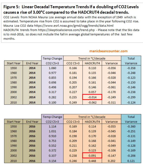
There are a number of things to observe from the trend data.

The most visual difference between the two tables is the first has a pause in global warming after 2002, whilst the second has a warming trend. This is attributable to the impact of El Nino. These experts are also right in that it makes very little difference to the long term trend. If the long term is over 40 years, then it is like adding 0.04C per century that long term trend.

But there is far more within the tables than this observations. Concentrate first on the three “Trend in °C/decade” columns. The first is of the CO2 warming impact from figure 3. For a given end year, the shorter the period the higher is the warming trend. Next to this are Skeptical Science trends for the HADCRUT4 data set. Start Year 1960 has a higher trend than Start Year 1950 and Start Year 1970 has a higher trend than Start Year 1960. But then each later Start Year has a lower trend the previous Start Years. There is one exception. The period 2010 to 2016 has a much higher trend than for any other period – a consequence of the extreme El Nino event. Excluding this there are now over three decades where the actual warming trend has been diverging from the theory.

The third of the “Trend in °C/decade” columns is simply the difference between the HADCRUT4 temperature trend and the expected trend from rising CO2 levels. If a doubling of CO2 levels did produce around 3C of warming, and other greenhouse gases were also contributing to warming then one would expect that CO2 would eventually start explaining less than the observed warming. That is the variance would be positive. But CO2 levels accelerated, actual warming stalled, increasing the negative variance.


4. Putting the claims into context

Compare David Rose

Stunning new data indicates El Nino drove record highs in global temperatures suggesting rise may not be down to man-made emissions

With Climate Feedback KEY TAKE-AWAY

1.Recent record global surface temperatures are primarily the result of the long-term, human-caused warming trend. A smaller boost from El Niño conditions has helped set new records in 2015 and 2016.

The HADCRUT4 temperature data shows that there had been no warming for over a decade, following a warming trend. This is in direct contradiction to theory which would predict that CO2-based warming would be at a higher rate than previously. Given that a record temperatures following this hiatus come as part of a naturally-occurring El Nino event it is fair to say that record highs in global temperatures ….. may not be down to man-made emissions.

The so-called long-term warming trend encompasses both the late twentieth century warming and the twenty-first century hiatus. As the later flatly contradicts theory it is incorrect to describe the long-term warming trend as “human-caused”. There needs to be a more circumspect description, such as the vast majority of academics working in climate-related areas believe that the long-term (last 50+ years) warming  is mostly “human-caused”. This would be in line with the first bullet point from the UNIPCC AR5 WG1 SPM section D3:-

It is extremely likely that more than half of the observed increase in global average surface temperature from 1951 to 2010 was caused by the anthropogenic increase in greenhouse gas concentrations and other anthropogenic forcings together.

When the IPCC’s summary opinion, and the actual data are taken into account Zeke Hausfather’s comment that the records “are primarily because of a long-term warming trend driven by human emissions of greenhouse gases” is dogmatic.

Now consider what David Rose said in the second article

El Nino is not caused by greenhouse gases and has nothing to do with climate change. It is true that the massive 2015-16 El Nino – probably the strongest ever seen – took place against a steady warming trend, most of which scientists believe has been caused by human emissions.

Compare this to Kyle Armour’s statement about the first article.

It is well known that global temperature falls after receiving a temporary boost from El Niño. The author cherry-picks the slight cooling at the end of the current El Niño to suggest that the long-term global warming trend has ended. It has not.

This time Rose seems to have responded to the pressure by stating that there is a long-term warming trend, despite the data clearly showing that this is untrue, except in the vaguest sense. There data does not show a single warming trend. Going back to the skeptical science trends we can break down the data from 1950 into four periods.

1950-1976 -0.014 ±0.072 °C/decade (2σ)

1976-2002 0.180 ±0.068 °C/decade (2σ)

2002-2014 -0.014 ±0.166 °C/decade (2σ)

2014-2016 1.889 ±1.882 °C/decade (2σ)

There was warming for about a quarter of a century sandwiched between two periods of no warming. At the end is an uptick. Only very loosely can anyone speak of a long-term warming trend in the data. But basic theory hypotheses a continuous, non-linear, warming trend. Journalists can be excused failing to make the distinctions. As non-experts they will reference opinion that appears sensibly expressed, especially when the alleged experts in the field are united in using such language. But those in academia, who should have a demonstrable understanding of theory and data, should be more circumspect in their statements when speaking as experts in their field. (Kyle Armour’s comment is an extreme example of what happens when academics completely suspend drawing on their expertise.)  This is particularly true when there are strong divergences between the theory and the data. The consequence is plain to see. Expert academic opinion tries to bring the real world into line with the theory by authoritative but banal statements about trends.
Kevin Marshall

£319 billion on Climate Change for approximately nothing

The major reason for abandoning the Climate Change Act 2008 is not due to the massive financial burden imposed on families, but because it will do approximately nothing to curb global greenhouse gas emissions. Massive costs are being imposed for near zero prospective benefit.

At the weekend the GWPF published a paper by Peter Lilley MP on the costs of The Climate Change Act 2008. From 2014 to 2030 he estimates a total cost of £319 billion to ensure that in 2030 British greenhouse gas emissions are 57% below their 1990 levels.
Putting this into context, listen to then Environment Minister David Miliband introducing the Climate Change Bill in 2007.

The 2008 Act increased the 2050 target from 60% to 80%. Miliband recognizes that what the UK does is not sufficient to stop a global problem. That requires a global solution. Rather, the aim is for Britain to lead the way, with other industrialized countries encouraged to follow. The developing countries are given a free choice of “a low carbon path of development rather than to repeat the mistakes of the industrialized countries.

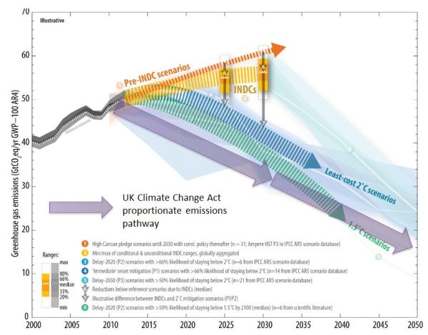
Over eight years after the little video was made and seven years after the Climate Change Act was passed (with an increased 2050 emissions reduction target of 80% reduction on 1990 levels) was the COP21 in Paris. The responses from other countries to Britain’s lead were in the INDC submission, which the UNFCCC summarized in a graph, and I have annotated.

The UNFCCC have four bands. First, in orange, is the Pre-INDC scenarios. Then in yellow is the projected global impact if all the vague policy proposals are full enacted. In blue is the least cost 2◦C pathway for global emissions reductions, whilst in green is the least cost 1.5◦C pathway.

I have superimposed lilac arrows showing the UK Climate Act proportionate emissions pathway achieving a 57% emissions reduction by 2030 and an 80% emissions reduction by 2050 compared to the baseline 1990 emissions. That is, if all countries were to follow Britain’s lead, then the 2◦C warming limit would not be breached.

What this clearly shows is that collectively countries have not followed Britain’s lead. Even if the policy proposals were fully enacted (an unlikely scenario) the yellow arrow quite clearly shows that global emissions will still be rising in 2030.

This needs to be put into context of costs and benefits. The year before David Miliband launched the Climate Bill the Stern Review was published. The Summary of Conclusions gave the justification for reducing greenhouse emissions.

Using the results from formal economic models, the Review estimates that if we don’t act, the overall costs and risks of climate change will be equivalent to losing at least 5% of global GDP each year, now and forever. If a wider range of risks and impacts is taken into account, the estimates of damage could rise to 20% of GDP or more. In contrast, the costs of action – reducing greenhouse gas emissions to avoid the worst impacts of climate change – can be limited to around 1% of global GDP each year.

Britain is spending the money to avert catastrophic global warming, but future generations will still be subjected to costs of climate catastrophe. It not much worse in terms of wasting money if the Stern Review grossly exaggerated the likely costs of warming and massively understated the policy costs, as Peter Lilley and Richard Tol laid out in their recent paper “The Stern Review : Ten Years On“.

However, if the British Government had conducted some proper assessment of the effectiveness of policy (or the Opposition has done their job in holding the Government to account) then it would have been clear that sufficient countries would never follow Britain’s lead. Last year Robin Guenier published some notes on Supreme Court Justice Phillip Sands lecture CLIMATE CHANGE and THE RULE OF LAW. Guenier stated of the Rio Declaration of 1992

There’s little, if any, evidence that the undoubted disagreements about the science – the focus of Professor Sands’ concern in his lecture – are the reason it’s proving so difficult to come to an effective agreement to restrict GHG emissions. In contrast however, the Annex I / non-Annex I distinction has had huge consequences. These arise in particular from Article 4.7:

“The extent to which developing country Parties will effectively implement their commitments under the Convention … will take fully into account that economic and social development and poverty eradication are the first and overriding priorities of the developing country Parties.” [My emphasis]

When the Convention was enacted (1992) the effective exemption of developing countries from environmental constraint made some sense. But over the years Non-Annex I countries, which include major economies such as China, India, South Korea, Brazil, South Africa, Saudi Arabia and Iran, have become increasingly powerful: in 2012 responsible for 67% of global CO2 emissions.

Robin Guenier uses estimates for CO2 emissions not (the admittedly harder to estimate) GHG emissions, of which CO2 comprises about two-thirds. But estimates are available from from the European Commission’s “Emissions Database for Global and Atmospheric Research” (EDGAR) for the period 1990 to 2012. I divided up the emissions between the Annex countries and the Non-Annex countries. 

The developing countries accounted for 64% of global GHG emissions in 2012, up from 47% in 1990 and 57% in 2005 when the Stern Review was being written. From 1990 to 2012 global emissions increased by 41% or 15,700 MtCO2e, whilst those of the Non-Annex countries increased by 90% or 16,400 MtCO2e  to 34,600 MtCO2e. The emissions in the United Kingdom decreased in the period (mostly for reasons other than mitigation policies) by 25% to 586 MtCO2e or 1.1% of the estimated global total.

It would have been abundantly clear to anyone who actually looked at the GHG emissions figures by country that the Rio Declaration 1992 was going to prevent any attempt to significantly reduce global GHG emissions. Since 1992 the phenomenal economic growth of countries like China and India, driven by the low energy costs of fossil fuels, have made the impossibility of reducing global emissions even starker. Yet still the IPCC, UNFCCC, many Governments and a large Academic consensus have failed to acknowledge, let alone understand, the real world data. Still they talk about reducing global emissions by over 80% in a couple of generations. In terms of the United Kingdom, the INDC submissions produced last year should have been further confirmation that the Government has no rational justification for imposing the massive costs on families, increasing inequalities and destroying jobs in the process.

Kevin Marshall


The Climate Alarmist Reaction to a Trump Presidency

A few weeks ago cliscep had a piece Trump, climate and the future of the world that looked at the immediate reactions to the surprise victory in the US Presidential election amongst the climate community. Brad Keyes noted Jo Romm’s piece will President Trump pull the plug on a livable climate?. To support this Romm stated

Indeed, one independent firm, Lux Research, projected last week that “estimated emissions would be 16 percent higher after two terms of Trump’s policies than they would be after two terms of Clinton’s, amounting to 3.4 billion tons greater emissions over the next eight years.”

There is a little graph to sort of back this up.

Whilst Romm then states two reasons why he does not think emissions will rise so much (Trump will cause a massive recession and will not win a second term) he then states the Twitter quote:-

That said, the damage and delay that even a one-term President Trump could do will make the already difficult task of keeping total warming well below 2°C essentially impossible.

So a difference of much less than 3.4 GtCO2e over eight years will make keeping total warming well below 2°C essentially impossible.
Before looking at the evidence that contradicts this, there are even more bizarre claims made by the expert climate scientists at RealClimate. They use a different graph which is probably a couple of years old and explain:-

Here are some numbers. Carbon emissions from the United States have been dropping since the year 2000, more than on-track to meet a target for the year 2020. Perhaps with continued effort and improving technology, emissions might have dropped to below the 2020 target by 2020, let’s say to 5 gigatons of CO2 per year (5000 megatons in the plot). In actuality, now, let’s say that removing restrictions on energy inefficiency and air pollution could potentially lead to US emissions by 2020 of about 7 gigatons of CO2. This assumes that future growth in emissions followed the faster growth rates from the 1990’s.
Maybe neither of these things will happen exactly, but these scenarios give us a high-end estimate for the difference between the two, which comes to about 4 gigatons of CO2 over four years. There will also probably be extra emissions beyond 2020 due to the lost opportunity to decarbonize and streamline the energy system between now and then. Call it 4-6 gigatons of Trump CO2.
This large quantity of gas can be put into the context of what it will take to avoid the peak warming threshold agreed to in Paris. In order to avoid exceeding a very disruptive warming of 1.5 °C with 66% probability, humanity can release approximately 220 gigatons of CO2 after January, 2017 (IPCC Climate Change 2014 Synthesis report, Table 2.2, corrected for emissions since 2011). The 4-6 Gtons of Trump CO2 will not by itself put the world over this threshold. But global CO2 emission rates are now about 36 gigatons of CO2 per year, giving a time horizon of only about six years of business-as-usual (!) before we cross the line, leaving basically no time for screwing around. To reach the catastrophic 2 °C, about 1000 gigatons of CO2 remain (about 20 years of business as usual). Note that these estimates were done before global temperatures spiked since 2014 — we are currently at 1.2 °C! So these temperature boundaries may be closer than was recently thought.

RealClimate come up with nearly twice the difference made by Joe Romm / Lux Research, but at least admit in the final paragraph that whoever won would not make much difference.
There are two parts to putting these analyses into context – the US context and the global one.
In the USA emissions have indeed been falling since 2000, this despite the population growing. The rate of decline has significantly increased in the years of the Obama Presidency, but for reasons quite separate from actions to reduce emissions. First there was the credit crunch, followed by the slowest recovery in US history. Second, the high oil price encouraged emissions reductions, along with the loss of energy-intensive industries to countries with lower energy costs. Third is that the shale gas revolution has meant switching from coal to gas in electricity production.
But the global context is even more important. RealClimate does acknowledge the global figure, but only mentions CO2 emissions. The 36GtCO2 is only two-thirds of total greenhouse gas emissions of about 55GTCO2e and that figure is rising by 1-2% a year. The graph – reproduced from the USA INDC submission to the UNFCCC – clearly states that it is in million tonnes of carbon dioxide equivalent. What is more, these are vague policy proposals, that President Obama would have been unable to get through Congress. Further, most of the proposed emission reductions were through extrapolating trends that of what has been happening without any policy intervention.
If the 1.5°C limit breached from 220 GtCO2e of additional emissions, it will be breached in the run-up to Christmas 2020. The 1000 GtCO2e for the 2°C limit was from 2011. By simple arithmetic it is now below 800GtCO2e with about 15 years remaining if (a) a doubling of CO2 levels (or equivalent GHG gases) leads to 3°C of warming (b) the estimated quantity of emissions to a unit rise in atmospheric gas levels is correct and (b) the GHG gas emitted is retained for a very long period in the atmosphere.
Even simple arithmetic is not required. Prior to the Paris talks the UNFCCC combined all the INDCs – including that of the USA to cut emissions as shown in the graph above – were globally aggregated and compared to the approximate emissions pathways for 1.5°C and least-cost 2°C warming. The updated version, post-Paris is below.

The difference Donald Trump will make is somewhere in the thickness of the thick yellow line. There is no prospect of the aimed-for blue emissions pathways. No amount of ranting or protests at the President-elect Trump will change the insignificant difference the United States will make with any politically-acceptable and workable set of policies, nor can make in a country with less than a twentieth of the global population and less that one seventh of global emissions.

Kevin Marshall

Update on a Global Carbon Tax

In a previous post I looked a statement made by Richard Tol in his recent paper The Structure of the Climate Debate

Only a modest carbon tax is needed to keep atmospheric concentrations below a high target but the required tax rapidly increases with the stringency of the target. If concentrations are to be kept below 450 ppm CO2eq, the global carbon tax should reach some $210/tCO2 in 2020 or so (Tol 2013).

Tol, to his credit, replied to me (and others) in the cliscep comments. In particular

Note that these climate policies consist of two components: An initial carbon tax, and its rate of increase (4-6% a year).

The $210 carbon tax in 2020 is just a starting point. With a 5% escalation, it would double every 14 years making the carbon tax $910 in 2050, $3070 in 2075 and $10,400 in 2100. The escalator is the far more important aspect in reducing demand for fossil fuels through a combination of reducing energy use and switching to more expensive (and often less convenient) renewable sources. The escalator was not clear in the original article, and Richard Tol has agreed to make a correction.

Consider again just imposing a fixed $210 carbon tax. From the British perspective the additional tax on petrol (gasoline), with 20% VAT applied, is equivalent to 47p a litre added to the retail price. The tax is already nearly 70p a litre, so unlikely to have the impact on motorists of reducing their consumption by 90% or more. Even with the tax at 200p a litre implied by a $910 t/CO2 tax (making petrol £3.13 a litre) may not achieve this objective. For a car doing 15000 miles at 39mpg, this would generate an additional cost to the owner of £3500 per year. It would still be less than the depreciation on a family car averaged over the first three years. It might also be less than the full costs of converting to electric cars, particularly if the roll-out was not subsidized on the purchase cost and provision of charging points. Within the UK, the carbon tax would also replace the current renewables policy. Here the escalator would really hit home. For coal-fired power stations producing 400kg CO2 per megawatt hour, the carbon tax would be £70Mwh in 2020 and £300Mwh in 2050. Gas-fired power stations would have a tax of about half that level. Even wind turbines, backed by massive pump-storage schemes would be much cheaper. Nuclear power would be the cheapest alternative of all. But British voters are hardly going to keep on voting for a Government that imposes real increases in taxes of five percent a year until they become unaffordable except for the very rich.

However, it is from the global perspective that the cost of the carbon tax really hits home. In another comment Tol says

The big worry for climate policy, studiously avoided by the majority of its advocates, is that you need lots of cheap energy in the early stages of economic development.

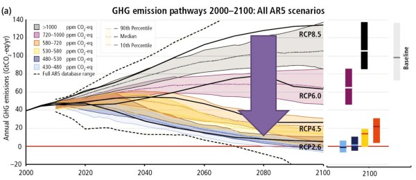
It is worth stating again that a Global Carbon Tax needs to be Global to achieve the desired objectives. From the UNIPCC AR5 Synthesis Report Summary for Policy Makers is graphic SPM11(a). This shows the non-policy or Business as Usual RCP8.5 scenario, where emissions in 2100 are projected to be over 2.5 times the level of 2010. The 2C warming target is the RCP2.6 scenario. I have inserted a big arrow to show the difference that the global carbon tax needs to make. It can be demonstrated that most of the emissions growth will come from the developing countries, following the pattern from at least 1990.


The scale of the harm of policy is by assuming that the $210 carbon tax is applied without any change in demand at all, using the estimated CO2 emissions from fossil fuels for 2013 from CDIAC and the IMF 2015 GDP figures for ballpark estimates.
Global CO2 emissions from fossil fuels were about 33.8 billion tonnes (two-thirds of total GHG emissions). A $210 carbon tax without any effect on demand would thus generate $7100 bn. This represents nearly 10% of global GBP of $73500bn. If we assume 2% emissions growth and 3% economic growth, then the carbon tax would represent 9.6% of GDP in 2020 without any drop in emissions.
Here is the same calculation for selected countries using 2013 emissions and GDP data.

30-33% Iran, Russia, South Africa
19-20% India, China
16-18% Thailand, Malaysia, Vietnam
11-14% Poland, Czech Republic, Pakistan, Egypt, Indonesia.
7% Bangladesh, Philippines
6-7% USA, Japan, Canada, Australia
4-5% Spain. Germany, Nigeria
UK 3.4% France 2.9%

The highest tax rates are a result of inefficient economic systems. Iran has subsidised petrol, effectively a negative carbon tax. South Africa’s high emissions are as a result of apartheid. Oil embargoes caused it to convert coal to liquids, a process that generates 4-5 times the CO2 of burning coal alone. Russia, in common with its neighbours, still has the legacy of the economically-inefficient communism.
The carbon tax would also be high as a proportion of GDP for the rapidly emerging economies. It highlights the Tol’s comment about needing lots of cheap energy in the early stages of economic development. With higher fossil fuel emissions per $1000 of GDP the impact on output would be relatively greater in the emerging economies than in the OECD. A globally uniform carbon tax would end up transferring back some manufacturing back to the more energy efficient economies, slowing economic growth and thus emissions growth.
More importantly, emerging countries have large parts of the population with very low energy consumption. Even those with access to gas and electricity have much lower energy consumption than is typical in the West, whether from heating, air conditioning, cooking, or private transport. Pushing up the cost of energy will massively slow down the spread of consumerism and consequent improvements in living standards.

Three years ago I looked at the takeaway policy quote from the Stern Review.

Using the results from formal economic models, the Review estimates that if we don’t act, the overall costs and risks of climate change will be equivalent to losing at least 5% of global GDP each year, now and forever. If a wider range of risks and impacts is taken into account, the estimates of damage could rise to 20% of GDP or more. In contrast, the costs of action – reducing greenhouse gas emissions to avoid the worst impacts of climate change – can be limited to around 1% of global GDP each year.

I largely agree with Richard Tol when he states that a carbon tax is the optimal policy in terms of maximum effect for minimum cost, at least with respect to fossil fuel emissions. Yet a high, and rapidly increasing, carbon tax would cost far more than 1% of global GDP each year, even if the additional tax revenue was spent efficiently and/or used to reduce other taxes. But the most pernicious effects would be felt in the effects on long-term economic growth – the very growth that is moving billions of people out of poverty towards the far better living standards we enjoy in the Western World. The  carbon tax does not present a feasible policy even in theory to achieve the objectives desired. Yet is, in theory, the best policy available.

Kevin Marshall

Results of Sea-Level Rise Extremism in Miami-Dade

A couple of years ago I posted* in response to a post on sea level rise at The Conversation

A senior geology professor in Miami, who also chairs the science committee for the Miami-Dade Climate Change Advisory Task Force, has views on future sea level rise that are way more extreme than the available evidence.

My Summary started

The claim by Professor Wanless at the Conversation that sea levels could rise by 1.25 to 2m by 2100 is way too extreme it is based on top-slicing the estimates on a NOAA 2012 report. The top-end estimates were not included by the UNIPCC in its AR5 Sept 2013 report. In fact, the UNIPCC report stated it had low-confidence in estimates of sea level rise above its top-end 0.82m.

The Task Force has now concluded. The Miami-Dade Climate Change website states

The Sea Level Rise Task Force, formed in July 2013, developed several important recommendations, which are being implemented in Miami-Dade County. The Task Force reviewed relevant data and prior studies and reports regarding the potential impact of sea level rise on public services and facilities, real estate, water and other ecological resources, and property and infrastructure.

The Introduction to the extensive report report states (with conversions into mm inserted):-

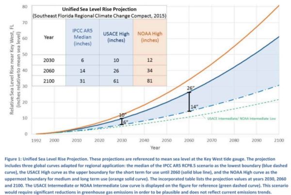
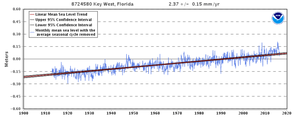
Since reliable record keeping began over 100 years ago at the tide gauge in Key West, the average sea level has risen approximately 228 millimeters (or 9 inches). This rise has been primarily due to thermal expansion (as warmer water occupies more volume) and to melting from glaciers and ice sheets. Over the next century, the rate of sea level rise is very likely to accelerate due to increased melting from land-based ice sheets, in particular Greenland. Recognizing the need for clear, consistent, and local information about future sea level rise projections, The Southeast Florida Regional Climate Change Compact developed the, “Unified Sea Level Rise Projection for Southeast Florida”. The updated projection, published in 2015, was developed by a panel of well-respected and informed scientists using the most recent and best available data. The projection (Figure 1) estimates that the region can expect to see average sea levels 6 to 10 inches (150 to 205 mm) higher by 2030 than they were in 1992, 14 to 34 inches (355 to 860 mm) higher by 2060, and 31 to 81 inches higher (790 to 2060 mm) by 2100. There is a more certain estimate for near-term changes and a greater uncertainty for estimates at the end of this century. This change in average sea levels will amplify the risks of storm surge and nuisance flooding.

This implies a massive acceleration in the rate of sea level-rise. In the last couple of years the rate of sea level rise has indeed accelerated. The NOAA data now shows a rate of 237 mm a century, by from 228 mm when the report was written. It is likely a blip and well with the margin of error.

To see how much sea level rise will have to accelerate to meet the forecasts, I will assume that from 1992 to 2015 the sea levels rose by 60 mm (2.4 inches) or 2.6 mm a year.

From 2016 to 2030 sea levels will need to rise by 6 to 10 mm a year on average, or about three or four times the current rate.

From 2016 to 2060 sea levels will need to rise by 8.5 to 23 mm a year on average, or about three or nine times the current rate.

From 2016 to 2100 sea levels will need to rise by 8.5 to 23.5 mm a year on average, or about three or nine times the current rate.

The impact of Professor Wanless on the Committee’s output should be clearly seen. A straight line forecast would be a 8 to 9 inch sea level rise by 2100. Many of the recommendations for planning will be based on a 2 foot 6 inch rise to a 6 foot 6 inch rise. Any reasonable person should take a measure to the Miami-Dade area – which is very low-lying and imagine the difference between a dyke 12 inches high and a dyke seven feet high along the Miami sea front.

Alternatively imagine the effect on property prices in Miami-Dade (2.6 million) and on neighbouring Broward and Palm Beach (3.1 million) if people really swallowed this whole. The tiny community of Fairbourne (724 people) in West Wales have had their properties made virtually value-less by a Welsh Government report and the alarmist reporting by the BBC.

*Thanks to Paul Homewood for a reminder to update my earlier post in his look at false alarmism on sea level rise in the Thames Estuary.

Kevin Marshall

Richard Tol on a Global Carbon Tax

Richard Tol, one of the World’s leading economists on climate, has just had published The Structure of the Climate Debate, a paper that makes some very good comments on the gulf between optimal policy and the reality of ineffective policy backed by a great army of bureaucrats, rent-seeking politicians and environmentalists who exaggerate the issues. It is this optimal policy  – a global carbon tax to constrain warming to 2C – that I take issue with. Both economic theory and the empirical evidence contradict this.  The following is a comment posted at cliscep

Richard Tol states in his paper

Only a modest carbon tax is needed to keep atmospheric concentrations below a high target but the required tax rapidly increases with the stringency of the target. If concentrations are to be kept below 450 ppm CO2eq, the global carbon tax should reach some $210/tCO2 in 2020 or so (Tol 2013).

The 450 ppm CO2eq, would produce 2C of warming from pre-industrial levels if a doubling of CO2 on its own produces 3C of warming. The UNFCCC produced a graph for COP21 to illustrate the global emissions pathway needed to ensure 2C limit :-

Whereas even with the all the vague policy proposals fully implemented global emissions will be about 10% higher in 2030 than in 2010, the 2C pathway has emissions 10-30% lower. That means a carbon tax of $210/tCO2 (now £170) would have to turn around the global relentless rise in emissions and have them falling rapidly. I am deeply sceptical that such a global policy would achieve anything like the that difference would be achieved even with an omnipotent, omniscient, and omnipresent planner to impose the tax. The reasons for that scepticism can be found by applying the tax to real world examples.
First let us apply a £170/tCO2 carbon tax to petrol, which produces 2.30kg of CO2 per litre. With 20% VAT applied is equivalent to 47p a litre added to the retail price. (Current excise duties with VAT are equivalent to £300/tCO2, the diesel £250/tCO2). For a car doing 15000 miles at 39mpg, this would generate an additional cost to the owner of £820 per year. Maybe a 15-30% increase in the full costs of running a small car in the UK. There is plenty of empirical visence of the effect of the oil price movements in the last couple of decades (especially in the period 2004-2008 when the price increased) to show that costs increases will have a much smaller effect on demand, whereas for the carbon tax to be effective it would need to have a much greater impact than the percentage cost increase.
Second, let us apply a $210/tCO2 carbon tax to coal-fired power stations. They produce about 400kg of CO2 per megawatt, so the cost would rise by $84MWH. In China, coal-fired electricity will retail at less than $30 MwH. China would rapidly switch to nuclear power. Even so, its power generation emissions might not start falling for at least a decade. Alternatively it might switch to gas, where the carbon tax would be half that of coal.
However, there is another lesson from oil prices, this time over the last three years. A small fall in demand leads to large falls in price, in the short term. That is the market responds by offsetting the cost of the global carbon tax. To use terms of basic economics the demand for fossil fuels is highly inelastic with respect to changes in price, and the supply of fossil fuels in the short term is highly inelastic to changes in demand.  Emissions reductions policies have not just turned out to be pretty useless in practice, they are pretty useless in theory (with real world political constraints removed) as well.

Kevin Marshall


Failed Arctic Sea Ice predictions illustrates Degenerating Climatology

The Telegraph yesterday carried an interesting article. Telegraph Experts said Arctic sea ice would melt entirely by September 2016 – they were wrong

Dire predictions that the Arctic would be devoid of sea ice by September this year have proven to be unfounded after latest satellite images showed there is far more now than in 2012.
Scientists such as Prof Peter Wadhams, of Cambridge University, and Prof Wieslaw Maslowski, of the Naval Postgraduate School in Moderey, California, have regularly forecast the loss of ice by 2016, which has been widely reported by the BBC and other media outlets.

In June, Michel at Trustyetverify blog traced a number of these false predictions. Michel summarized

(H)e also predicted until now:
• 2008 (falsified)
• 2 years from 2011 → 2013 (falsified)
• 2015 (falsified)
• 2016 (still to come, but will require a steep drop)
• 2017 (still to come)
• 2020 (still to come)
• 10 to 20 years from 2009 → 2029 (still to come)
• 20 to 30 years from 2010 → 2040 (still to come).

The 2016 prediction is now false. Paul Homewood has been looking at Professor Wadhams’ failed prophesies in a series of posts as well.

The Telegraph goes on to quote from three, more moderate, sources. One of them is :-

Andrew Shepherd, professor of earth observation at University College London, said there was now “overwhelming consensus” that the Arctic would be free of ice in the next few decades, but warned earlier predictions were based on poor extrapolation.
“A decade or so ago, climate models often failed to reproduce the decline in Arctic sea ice extent revealed by satellite observations,” he said.
“One upshot of this was that outlier predictions based on extrapolation alone were able to receive wide publicity.
“But climate models have improved considerably since then and they now do a much better job of simulating historical events.
This means we have greater confidence in their predictive skill, and the overwhelming consensus within the scientific community is that the Arctic Ocean will be effectively free of sea ice in a couple of decades should the present rate of decline continue.

(emphasis mine)

Professor Shepard is saying that the shorter-term (from a few months to a few years) highly dire predictions have turned out to be false, but improved techniques in modelling enable much more sound predictions over 25-50 years to be made. That would require a development on two dimensions – scale and time. Detecting a samll human-caused change over decades needs far greater skill in differentiating from natural variations on a year-by-year time scale from a dramatic shift. Yet it would appear that at the end of the last century there was a natural upturn following from an unusually cold period in the 1950s to the 1970s, as documented by HH Lamb. This resulted in an extension in the sea ice. Detection of the human influence problem is even worse if the natural reduction in sea ice has worked concurrently with that human influence. However, instead of offering us demonstrated increased technical competency in modelling (as opposed to more elaborate models), Professor Shepard offers us the consensus of belief that the more moderate predictions are reliable.
This is a clear example of degenerating climatology that I outlined in last year. In particular, I proposed that rather than progressive climate science – increasing scientific evidence and more rigorous procedures for tighter hypotheses about clear catastrophic anthropogenic global warming – we have degenerating climatology, which is ever weaker and vaguer evidence for some global warming.

If Professor Wadhams had consistently predicted the lack of summer sea ice for a set time period, then it would be strong confirmation of a potentially catastrophic problem. Climatology would have scored a major success. Even if instead of ice-free summers by now, there had been evidence of clear acceleration in the decline in sea ice extent, then it could have been viewed as some progression. But instead we should accept a consensus of belief that will only be confirmed or refuted decades ahead. The interpretation of success or failure. will then, no doubt, be given to the same consensus who were responsible for the vague predictions in the first place.

Kevin Marshall

Jeremy Corbyn needs to do the Maths on Boundary Commission Proposals

In my previous post I noted how some Labour MPs were falsely claiming that the Boundary Commission’s recommendations for England and Wales were party-political gerrymandering. Labour Party Leader, the Rt Hon Jeremy Corbyn MP makes a quite different claim to some of his more desperate MPs.

Corbyn claims that since last December (which the Boundary Commission used as a basis of the boundary changes) the electorate has grown by two million people. That is nearly 5% of the electorate. As a result of the wrong figures “you cannot deliver a fair and democratic result on the basis of information that is a year out of date.
Actually it is possible for it to be fair and democratic if the growth in the electorate is evenly spread across the country. That should be a default position that Corbyn needs to disprove. The question is, how much would the imbalance have to be to wipe out the disadvantage Labour gets from the boundary review – a disadvantage due to current 231 Labour seats in England and Wales having on average 3515 fewer constituents than the 329 Conservative seats in May 2015. Let us do the maths, ignoring the 13 seats held by other parties and the Speaker. To even up average constituency size Labour constituencies would need about 812,000 extra voters (231 x 3515), and for the rest of the two million to be evenly spread between the other 560 constituencies. That is about 2120 extra voters. It is not impossible that the average Labour constituency has added 5635 to the electoral roll (>8% extra) and the average Conservative constituency has added 2120 to the electoral roll (<3% extra). Winning the millions on Lotto is not impossible either. But both are highly unlikely, as the reason for the Boundary Review is that Constituency sizes have diverged, with greater growth in the South of England than in the North of England and Wales. So like other Labour MPs, Jeremy Corbyns’ opposition to the Boundary Commission’s proposals seem to be opposition to greater equality and fairness in the British democratic processes.
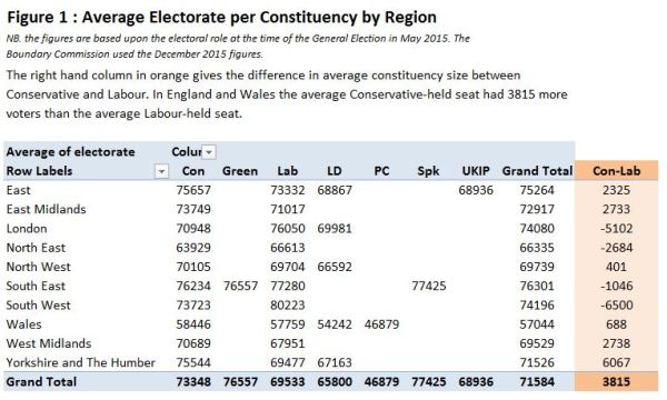
Two graphs to illustrate this point. Figure 1 from the previous post shows the average constituency size by party and region.

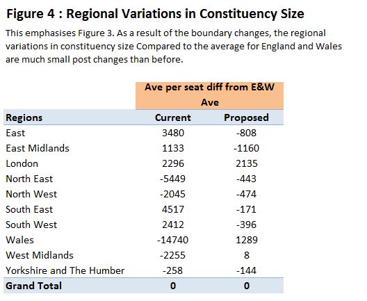
Figure 4 from the previous post shows that average constituency size per region is made much closer to the average constituency size for England and Wales in the proposed changes.


Kevin Marshall

Are the Proposed Boundary Changes Designed to hurt the Labour Party?

Yesterday the proposed new boundaries for England and Wales were published by the Boundary Commission. Nationally the total number of constituencies will be reduced from 650 to 600, still leaving Britain with one of the largest number of representatives of any democratic parliament. In England the reduction is from 533 to 501 and in Wales from 40 to 29. The UK Polling Report website reports

The changes in England and Wales result in the Conservatives losing 10 seats, Labour losing 28 seats, the Liberal Democrats losing 4 and the Greens losing Brighton Pavilion (though notional calculations like these risk underestimating the performance of parties with isolated pockets of support like the Greens and Lib Dems, so it may not hit them as hard as these suggest).

The Guardian Reports under the banner Boundary changes are designed to hurt us at next election, says Labour MP

Jon Ashworth, the shadow Cabinet Office minister leading the process for Labour, said the party was convinced the proposals were motivated by party politics.

The Manchester Evening News carries this comment

Jonathan Reynolds, Labour MP for Stalybridge and Hyde, accused the Conservatives of ‘old-fashioned gerrymandering’.
I will contest these proposals, because I believe they are a naked attempt to increase the electoral prospects of the Conservative Party at the expense of coherent parliamentary representation,” he said.

This are quite a serious claim to make, particularly as the Boundary Commission clearly states

The Boundary Commission for England is the independent and impartial body that is considering where the boundaries of the new constituencies should be. We must report to Parliament in September 2018.
In doing so, we have to ensure that every new constituency has roughly the same number of electors: no fewer than 71,031 and no more than 78,507. While proposing a set of boundaries which are fairer and more equal, the Commission will also try to reflect geographic factors and local ties. The Commission will also look at the boundaries of existing constituencies and local government patterns in redrawing the map of parliamentary constituency boundaries across England.
In undertaking the 2018 Review, we rely heavily on evidence from the public about their local area. Though we have to work within the tight electorate thresholds outlined above, we seek to recommend constituency boundaries that reflect local areas as much as we can. You can find more detailed guidance in our Guide to the 2018 Review.

I thought I would look at the figures myself to see whether the Boundary Commission has done a fair job overall, or has basically lied, providing a deliberately partisan result, that the UK Polling Report has been complicit in supporting.
For previous posts I downloaded the results of the May 2015 General Election by constituency. I then spilt the results into the regions of England and Wales.
Figure 1 shows the average size of constituency by Region and Party. Spk is the Speaker of the House of Commons.

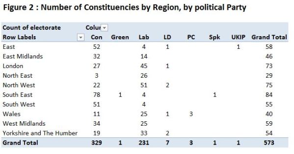
On average the Conservative held constituencies had 3815 more voters in than Labour held ones. But there are large regional differences. Figure 2 shows the number of constituencies by region and political party.

In the South East and South West, where Labour have larger average constituency sizes they have very few seats. In these regions, the regional average seat size is greater than the England and Wales average, so there will be proportionately less seat reductions. The Conservatives, with the vast majority of seats in these regions do not lose from a reduction in the national total and a more equitable distribution. In the East Midlands, West Midlands and Yorkshire and The Humber, Labour are well represented, but have smaller average seat sizes than the Conservatives. In the North West and in Wales Labour are well represented, the average seat sizes in Labour seats are similar to Conservative seats, but the regional average seat sizes are smaller than the England and Wales average. Smaller average seat sizes in these regions will hit Labour harder than the Conservatives due to Labour’s higher representation.
The only exception to the England and Wales picture is London. The region has larger than average constituencies at present, the average constituency size of Labour constituencies is bigger than Conservative constituencies and over 60% of the 73 constituencies are Labour held. But still the region and Labour lose seats, though proportionately less than elsewhere.
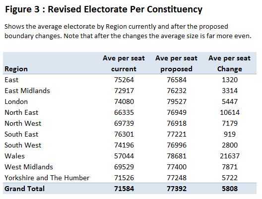
The effect of the revisions in shown in the average seat size. In Figure 3 with less seats the average seat size increases, but in some regions by far more than others, resulting in much less regional variation from the proposed boundary changes.

Figure 4 emphasizes the more even distribution of seat size. Currently, the variation of average constituency by region from England and Wales average is between -14740 (Wales) and +4517 (South East). Under the proposals, the variation is between -1160 (East Midlands) and + 2135 (London). https://manicbeancounter.com/wp-content/uploads/2016/09/fig4variationewave.jpg

In London’s case it could be argued for another two constituencies, but this is hardly significant. Also, given that London MPs spend their week far nearer to their constituents than any other region, an extra 2-3% of people to represent is hardly a burden.
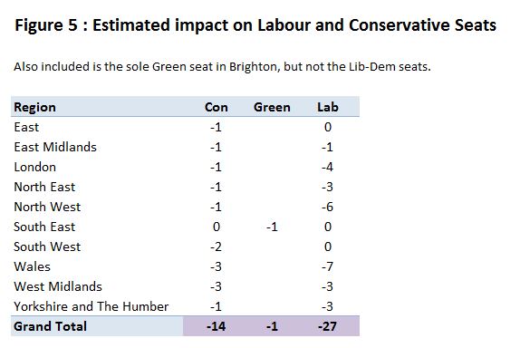
Finally I have done my own estimated impact on Labour, Conservative and Green seats based on changes in regional seat average sizes in Figure 5. If though I do not include the Lib-Dems, the results are very similar to UK Polling Report. The much more even (and therefore fairer) distribution of seats, along with a modest reduction in the total, disadvantages the Labour Party far more than the Conservatives, despite having two-thirds of the seats.

The Labour Party MPs who are doubting the independence of the Boundary Commission should apologize. The evidence is clearly against them.

Kevin Marshall

Going for Brexit or denying the EU Referendum

The Rt Hon David Davies MP and Secretary of State for Exiting the EU gave an update to the House of Commons today. He made quite clear what Brexit means

Naturally, people want to know what Brexit will mean.
Simply, it means the UK leaving the European Union. We will decide on our borders, our laws, and taxpayers’ money.
It means getting the best deal for Britain – one that is unique to Britain and not an ‘off the shelf’ solution. This must mean controls on the numbers of people who come to Britain from Europe – but also a positive outcome for those who wish to trade in goods and services.

He went on to lay out the principles on which Britain would proceed.

…as we proceed, we will be guided by some clear principles. First, as I said, we wish to build a national consensus around our position. Second, while always putting the national interest first, we will always act in good faith towards our European partners. Third, wherever possible we will try to minimise any uncertainty that change can inevitably bring. And, fourth, crucially, we will – by the end of this process – have left the European Union, and put the sovereignty and supremacy of this Parliament beyond doubt.

On other words Britain will Brexit is in a very British fashion.

– It will be from principles, not from specific objectives or adhering to specific rules.
– Britain will act honourably, something that the British have long been known for commercial dealings.
– It will recognize that other EU members have interests as well. The outcome being aimed for is where Britain’s relationship to the EU is based on co-operation and trade where both sides are net winners.
– At the end of the process Britain will have a more sovereign Parliament. That is, the democratically elected Government will be able to decide the future course of country, for better or worse.

Text is at ConservativeHome
Emily Thornberry MP, speaking for the Labour Party, gave a somewhat different perspective from about 13:10

– Strategy consists of clearly laid out and concrete plan.
– There are areas of policy that should placed outside of the scope of a sovereign Parliament, such “workers rights” and guarantees for EU Nationals currently resident in the UK.
– A “positive vision” consists of definite objectives.
– You listen to outside gloomy prophesies that support your perspective.
– The Government are now rushing to start negotiation, without a well-thought plan. Given that the Government is delaying triggering Article 50 until 2017, the means she is wanting a slower pace. But on 24th June when the referendum result was announced, Labour Leader Jeremy Corbyn was all for triggering Article 50 straight away. Is this another open split with the Labour Leader, or an about-face in Labour policy?
– Article 50 should not be triggered without a parliamentary vote to authorize.

On triggering Article 50 David Davies pointed out 20.35 there was a referendum bill that went through the House of Commons, and was voted for 6 to 1. Emily Thornberry voted in favour. It was made perfectly clear by the then Foreign Secretary at the time that the EU referendum was not a consultation, or an advice to parliament, but a decision by the electorate. The words of the Act do not state that, but people were lead to believe that in the campaign. Most importantly Will Straw, leader of Britain Stronger in Europe (the official Remain campaign) said the decision was for the voters.

RE: THE FACTS YOU NEED TO KNOW ABOUT EU AND THE REFERENDUM
On 23rd June you will get to vote on the EU Referendum and decide whether Britain remains in or leaves Europe.

Apart from the inaccuracy of naming the decision as whether to leave the geographical continent rather than the political organisation, the statement could not be clearer. Yet the losers in the Referendum want to re-interpret the meaning of the result.

Kevin Marshall