Study on UK Wind and Solar potential fails on costs

Oxford University’s Smith School of Enterprise and the Environment in August published a report “Could Britain’s energy demand be met entirely by wind and solar?“, a short briefing “Wind and solar power could significantly exceed Britain’s energy needs” with a press release here. Being a (slightly) manic beancounter, I will review the underlying assumptions, particularly the costs.

Summary Points

  • Projected power demand is likely high, as demand will likely fall as energy becomes more expensive.
  • Report assumes massively increased load factors for wind turbines. A lot of this increase is from using benchmarks contingent on technological advances.
  • The theoretical UK scaling up of wind power is implausible. 3.8x for onshore wind, 9.4x for fixed offshore and >4000x for floating offshore wind. This to be achieved in less than 27 years.
  • Most recent cost of capital figures are from 2018, well before the recent steep rises in interest rates. Claim of falling discount rates is false.
  • The current wind turbine capacity is still a majority land based, with a tiny fraction floating offshore. A shift in the mix to more expensive technologies leads to an 82% increase in average levelised costs. Even with the improbable load capacity increases, the average levilised cost increase to 37%.
  • Biggest cost rise is from the need for storing days worth of electricity. The annual cost could be greater than the NHS 2023/24 budget.
  • The authors have not factored in the considerable risks of diminishing marginal returns.

Demand Estimates

The briefing summary states

299 TWh/year is an average of 34 GW, compared with 30 GW average demand in 2022 at grid.iamkate.com. I have no quibble with this value. But what is the five-fold increase by 2050 made-up of?

From page 7 of the full report.

So 2050 maximum energy demand will be slightly lower than today? For wind (comprising 78% of potential renewables output) the report reviews the estimates in Table 1, reproduced below as Figure 1

Figure 1: Table 1 from page 10 of the working paper

The study has quite high estimates of output compared to previously, but things have moved on. This is of course output per year. If the wind turbines operated at 100% capacity then the required for 24 hours a day, 365.25 days a year would be 265.5 GW, made up of 23.5GW for onshore, 64GW for fixed offshore and 178GW for floating offshore. In my opinion 1500 TWh is very much on the high side, as demand will fall as energy becomes far more expensive. Car use will fall, as will energy use in domestic heating when the considerably cheaper domestic gas is abandoned.

Wind Turbine Load Factors

Wind turbines don’t operate at anything like 100% of capacity. The report does not assume this. But it does assume load factors of 35% for onshore and 55% for offshore. Currently floating offshore is insignificant, so offshore wind can be combined together. The UK Government produces quarterly data on renewables, including load factors. In 2022 this average about 28% for onshore wind (17.6% in Q3 to 37.6% in Q1) and 41% for offshore wind (25.9% in Q3 to 51.5% in Q4). This data, shown in four charts in Figure 2 does not seem to shown an improving trend in load capacity.
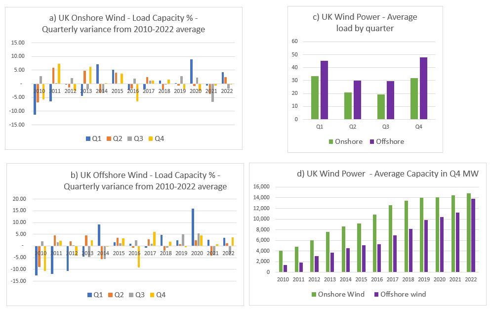
Figure 2 : Four charts illustrating UK wind load capacities and total capacities

The difference is in the report using benchmark standards, not extrapolating from existing experience. See footnote 19 on page 15. The first ref sited is a 2019 DNV study for the UK Department for Business, Energy & Industrial Strategy. The title – “Potential to improve Load Factor of offshore wind farms in the UK to 2035” – should give a clue as to why benchmark figures might be inappropriate to calculate future average loads. Especially when the report discusses new technologies and much larger turbines being used, whilst also assuming some load capacity improvements from reduced downtimes for maintenance.

Scaling up

The report states on page 10

From the UK Government quarterly data on renewables, these are the figures for Q3 2022. Q1 2023 gives 15.2 GW onshore and 14.1 GW offshore. This offshore value was almost entirely fixed. Current offshore floating capacity is 78 MW (0.078 GW). This implies that to reach the reports objectives of 2050 with 1500 TwH, onshore wind needs to increase 3.8 times, offshore fixed wind 9.4 times and offshore floating wind over 4000 times. Could diminishing returns, in both output capacities and costs per unit of capacity set in with this massive scaling up? Or maintenance problems from rapidly installing floating wind turbines of a size much greater than anything currently in service? On the other hand, the report notes that Scotland has higher average wind speeds than “Wales or Britain”, to which I suspect they mean that Scotland has higher average wind speeds to the rest of the UK. If so, they could be assuming a good proportion of the floating wind turbines will be located off Scotland, where wind speeds are higher and therefore the sea more treacherous. This map of just 19 GW of proposed floating wind turbines is indicative.

Cost of Capital

On page 36 the report states

You indeed find these rates on “Table 2.7: Technology-specific hurdle rates provided by Europe Economics”. My quibble is not that they are 2018 rates, but that during 2008-2020 interests rates were at historically low levels. In a 2023 paper it should recognise that globally interest rates have leapt since then. In the UK, base rates have risen from 0.1% in 2020 to 5.25% at the beginning of August 2023. This will surely affect the discount rates in use.

Wind turbine mix

Costs of wind turbines vary from project to project. However, the location determines the scale of costs. It is usually cheaper to put up a wind turbine on land than fix it to a sea bed, then construct a cable to land. This in turn is cheaper than anchoring a floating turbine to a sea bed often in water too deep to fix to the sea bed. If true, moving from land to floating offshore will increase average costs. For this comparison I will use some 2021 levilized costs of energy for wind turbines from US National Renewable Energy Laboratory (NREL).

Figure 3 : Page 6 of the NREL presentation 2021 Cost of Wind Energy Review

The levilized costs are $34 MWh for land-based, $78 MWh for fixed offshore, and $133 MWh for floating offshore. Based on the 2022 outputs, the UK weighted average levilized cost was about $60 MWh. On the same basis, the report’s weighted average levilized cost for 2050 is about $110 MWh. But allowing for 25% load capacity improvements for onshore and 34% for offshore brings average levilized cost down to $82 MWh. So the different mix of wind turbine types leads to an 83% average cost increase, but efficiency improvements bring this down to 37%. Given the use of benchmarks discussed above it would be reasonable to assume that the prospective mix variance cost increase is over 50%, ceteris paribus.

The levilized costs from the USA can be somewhat meaningless for the UK in the future, with maybe different cost structures. Rather than speculating, it is worth understanding why the levilized cost of floating wind turbines is 70% more than offshore fixed wind turbines, and 290% more (almost 4 times) than onshore wind turbines. To this end I have broken down the levilized costs into their component parts.

Figure 3 : NREL Levilized Costs of Wind 2021 Component Breakdown. A) Breakdown of total costs B) Breakdown of “Other Capex” in chart A

Observations

  • Financial costs are NOT the costs of borrowing on the original investment. The biggest element is cost contingency, followed by commissioning costs. Therefore, I assume that the likely long-term rise interest rates will impact the whole levilized cost.
  • Costs of turbines are a small part of the difference in costs.
  • Unsurprisingly, operating cost, including maintenance, are significantly higher out at sea than on land. Similarly for assembly & installation and for electrical infrastructure.
  • My big surprise is how much greater the cost of foundations are for a floating wind turbine are than a fixed offshore wind turbine. This needs further investigation. In the North Sea there is plenty of experience of floating massive objects with oil rigs, so the technology is not completely new.

What about the batteries?

The above issues may be trivial compared to the issue of “battery” storage for when 100% of electricity comes from renewables, for when the son don’t shine and the wind don’t blow. This is particularly true in the UK when there can be a few day of no wind, or even a few weeks of well below average wind. Interconnectors will help somewhat, but it is likely that neighbouring countries could be experiencing similar weather systems, so might not have any spare. This requires considerable storage of electricity. How much will depend on the excess renewables capacity, the variability weather systems relative to demand, and the acceptable risk of blackouts, or of leaving less essential users with limited or no power. As a ballpark estimate, I will assume 10 days of winter storage. 1500 TWh of annual usage gives 171 GW per hour on average. In winter this might be 200 GW per hour, or 48000 GWh for 10 or 48 million Mwh. The problem is how much would this cost?

In April 2023 it a 30 MWh storage system was announced costing £11 million. This was followed in May by a 99 MWh system costing £30 million. These respectively cost £367,000 and £333,000 per MWh. I will assume there will be considerable cost savings in scaling this up, with a cost of £100,000 per MWh. Multiplying this by 48,000,000 gives a cost estimate of £4.8 trillion, or nearly twice the 2022 UK GDP of £2.5 trillion. If one assumes a 25 year life of these storage facilities, this gives a more “modest” £192 billion annual cost. If this is divided by an annual usage of 1500 TWh it comes out at a cost of 12.8p KWh. These costs could be higher if interest rates are higher. The £192 billion costs are more than the 2023/24 NHS Budget.

This storage requirement could be conservative. On the other hand, if overall energy demand is much lower, due to energy being unaffordable it could be somewhat less. Without fossil fuel backup, there will be a compromise between costs energy storage and rationing with the risk of blackouts.

Calculating the risks

The approach of putting out a report with grandiose claims based on a number of assumptions, then expecting the public to accept those claims as gospel is just not good enough. There are risks that need to be quantified. Then, as a project progresses these risks can be managed, so the desired objectives are achieved in a timely manner using the least resources possible. These are things that ought to be rigorously reviewed before a project is adopted, learning from past experience and drawing on professionals in a number of disciplines. As noted above, there are a number of assumptions made where there are risks of cost overruns and/or shortfalls in claimed delivery. However, the biggest risks come from the law of diminishing marginal returns, a concept that has been understood for over 2 00 years. For offshore wind the optimal sites will be chosen first. Subsequent sites for a given technology will become more expensive per unit of output. There is also the technical issue of increased numbers of wind turbines having a braking effect on wind speeds, especially under stable conditions.

Concluding Comments

Technically, the answer to the question “could Britain’s energy demand be met entirely by wind and solar?” is in the affirmative, but not nearly so positively at the Smith School makes out. There are underlying technical assumptions that will likely not be borne out with further investigations. However, in terms of costs and reliable power output, the answer is strongly in the negative. This is an example of where rigorous review is needed before accepting policy proposals into the public arena. After all, the broader justification of contributing towards preventing “dangerous climate change” is upheld in that an active global net zero policy does not exist. Therefore, the only justification is on the basis of being net beneficial to the UK. From the above analysis, this is certainly not the case.

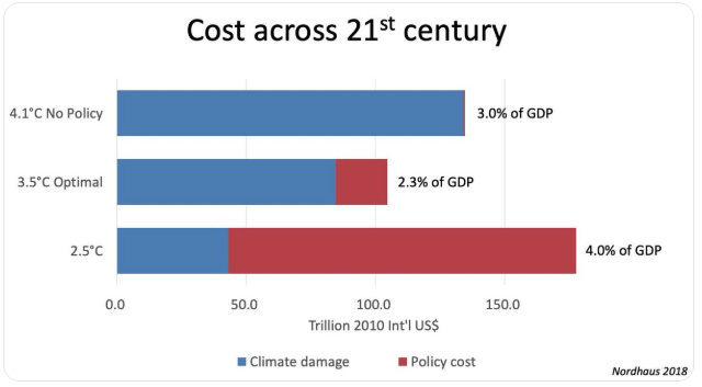
Nobel Laureate William Nordhaus demonstrates that pursuing climate mitigation will make a nation worse off

Summary

Nobel Laureate Professor William Nordhaus shows that the optimal climate mitigation policy is for far less mitigation than UNIPCCC proposes. That is to constrain warming by 2100 to 3.5°C instead of 2°C or less. But this optimal policy is based on a series of assumptions, including that policy is optimal and near universally applied. The current situation, with most countries without any effective mitigation policies, is that climate mitigation policies within a country will likely make that country worse off, even if they would be better off with the same policies were near universally applied. Countries applying costly climate mitigation policies are making their people worse off.

Context

Last week Bjorn Lomborg tweeted a chart derived from Nordhaus paper from August 2018 in the American Economic Review.

The paper citation is

Nordhaus, William. 2018. “Projections and Uncertainties about Climate Change in an Era of Minimal Climate Policies.” American Economic Journal: Economic Policy10 (3): 333-60.

The chart shows the optimal climate mitigation policy, based upon minimization of (a) the combined projected costs of climate mitigation policy and (b) residual net costs from human-caused climate change, is much closer to the non-policy option of 4.1°C than restraining warming to 2.5°C. By the assumptions of Nordhaus’s model greater warming constraint can only be achieved through much greater policy costs. The abstract concludes

The study confirms past estimates of likely rapid climate change over the next century if major climate-change policies are not taken. It suggests that it is unlikely that nations can achieve the 2°C target of international agreements, even if ambitious policies are introduced in the near term. The required carbon price needed to achieve current targets has risen over time as policies have been delayed.

A statement whose implications are ignored

This study is based on mainstream projections of greenhouse gas emissions and the resultant warming. Prof Nordhaus is in the climate mainstream, not a climate agnostic like myself. Given this, I find the opening statement interesting. (My bold)

Climate change remains the central environmental issue of today. While the Paris Agreement on climate change of 2015 (UN 2015) has been ratified, it is limited to voluntary emissions reductions for major countries, and the United States has withdrawn and indeed is moving backward. No binding agreement for emissions reductions is currently in place following the expiration of the Kyoto Protocol in 2012. Countries have agreed on a target temperature limit of 2°C, but this is far removed from actual policies, and is probably infeasible, as will be seen below.
The reality is that most countries are on a business-as-usual (BAU) trajectory of minimal policies to reduce their emissions; they are taking noncooperative policies that are in their national interest, but far from ones which would represent a global cooperative policy.

Although there is a paper agreement to constrain emissions commensurate with 2°C of warming, most countries are doing nothing – or next to nothing – to control their emissions. The real world situation is completely different to assumptions made in the model. The implications of this are skirted over by Nordhaus, but will be explored below.

The major results at the beginning of the paper are
  • The estimate of the SCC has been revised upward by about 50 percent since the last full version in 2013.
  • The international target for climate change with a limit of 2°C appears to be infeasible with reasonably accessible technologies even with very ambitious abatement strategies.
  • A target of 2.5°C is technically feasible but would require extreme and virtually universal global policy measures in the near future.

SCC is the social cost of carbon. The conclusions about policy are not obtained from understating the projected costs of climate change. Yet the aim to limit warming to 2°C appears infeasible. By implication limiting warming beyond this – such as to 1.5°C – should not be considered by rational policy-makers. Even a target of 2.5°C requires special conditions to be fulfilled and still is less optimal than doing nothing. The conclusion from the paper without going any further is achieving the aims of the Paris Climate Agreement will make the world a worse place than doing nothing. The combined costs of policy and any residual costs of climate change will be much greater than the projected costs of climate change.

Some assumptions

This outputs of a model are achieved by making a number of assumptions. When evaluating whether the model results are applicable to real world mitigation policy consideration needs to be given to whether those assumptions hold true, and the impact on policy if violated. I have picked some of the assumptions. The ones that are a direct or near direct quote, are in italics.

  1. Mitigation policies are optimal.
  2. Mitigation policies are almost universally applied in the near future.
  3. The abatement-cost function is highly convex, reflecting the sharp diminishing returns to reducing emissions.
  4. For the DICE model it is assumed that the rate of decarbonization going forward is −1.5 percent per year.
  5. The existence of a “backstop technology,” which is a technology that produces energy services with zero greenhouse gas (GHG) emissions.
  6. Assumed that there are no “negative emissions” technologies initially, but that negative emissions are available after 2150.
  7. Assumes that damages can be reasonably well approximated by a quadratic function of temperature change.
  8. Equilibrium climate sensitivity (ECS) is a mean warming of 3.1°C for an equilibrium CO2 doubling.

This list is far from exhaustive. For instance, it does not include assumptions about the discount rate, economic growth or emissions growth. However, the case against current climate mitigation policies, or proposed policies, can be made by consideration of the first four.

Implications of assumptions being violated

I am using a deliberately strong term for the assumptions not holding.

Clearly a policy is not optimal if it does not work, or even spends money to increase emissions. More subtle is using sub-optimal policies. For instance, raising the cost of electricity is less regressive the poor are compensated. As a result the emissions reductions are less, and there cost per tonne of CO2  mitigated rises. Or nuclear power is not favoured, so is replaced by a more expensive system of wind turbines and backup energy storage. These might be trivial issues if in general policy was focussed on the optimal policy of a universal carbon tax. No country is even close. Attempts to impose carbon taxes in France and Australia have proved deeply unpopular.

Given the current state of affairs described by Nordhaus in the introduction, the most violated assumption is that mitigation policy is not universally applied. Most countries have no effective climate mitigation policies, and very few have policies in place that are likely to result in any where near the huge global emission cuts required to achieve the 2°C warming limit. (The most recent estimate from the UNEP Emissions Gap Report 2018 is that global emissions need to be 25% lower in 2030 than in 2017). Thus globally the costs of unmitigated climate change will be close to the unmitigated 3% of GDP, with globally the policy costs being a small fraction of 1% of GDP. But a country that spends 1% of GDP on policy – even if that is optimal policy – will only see a miniscule reduction in its expected climate costs. Even the USA with about one seventh of global emissions, on Nordhaus’s assumptions efficiently spending 1% of output might expect future climate costs to fall by maybe 0.1%. The policy cost to mitigation cost for a country on its own is quite different to the entire world working collectively on similar policies. Assumption four of a reduction of 1.5% in global emissions illustrates the point in a slightly different way. If the USA started cutting its emissions by an additional 1.5% a year (they are falling without policy) then it would likely mean global emissions would keep on increasing.

The third assumption is another that is sufficient on its own to undermine climate mitigation. The UK and some States in America are pursuing what would be a less than 2°C pathway if it were universally applied. That means they are committing to a highly convex policy cost curve, (often made steeper by far from optimal policies) with virtually no benefits for future generations.

Best Policies under the model assumptions

The simplest alternative to climate mitigation policies could be to have no policies at all. However, if the climate change cost functions are a true representation, and given the current Paris Agreement this is not a viable option for those less thick-skinned than President Trump, or who have a majority who believe in climate change. Economic theory can provide some insights into the strategies to be employed. For instance if the climate cost curve is a quadratic as in Nordhaus (or steeper – in Stern I believe it was at least a quartic) there are rapidly diminishing returns to mitigation policies in terms of costs mitigated. For a politician who wants to serve their the simplest strategies are to

  • Give the impression of doing something to appear virtuous
  • Incur as little cost as possible, especially those that are visible to the majority
  • Benefit special interest groups, especially those with climate activist participants
  • Get other countries to bear the real costs of mitigation.

This implies that many political leaders who want to serve the best interests of their countries need to adopt a strategy of showing they are doing one thing to appear virtuous, whilst in reality doing something quite different.

In the countries dependent of extracting and exporting fossil fuels for a large part of their national income (e.g. the Gulf States, Russia, Kazakhstan, Turkmenistan etc.) different priorities and much higher marginal policy costs for global mitigation are present. In particular, if, as part of climate policies other countries were to shut down existing fossil fuel extraction, or fail to develop new sources of supply to a significant extent then market prices would rise, to the benefit of other producers.

Conclusion

Using Nordhaus’s model assumptions, if the World as a whole fulfilled the Paris Climate Agreement collectively with optimal policies, then the world would be worse off than if it did nothing. That is due to most countries pursuing little or no actual climate mitigation policies. Within this context, pursuing any costly climate mitigation policies will make a country worse off than doing nothing.

Assuming political leaders have the best interests of their country at heart, and regardless of whether they regard climate change a problem, the optimal policy strategy is to impose as little costly policy as possible for maximum appearance of being virtuous, whilst doing the upmost to get other countries to pursue costly mitigation policies.

Finally

I reached the conclusion that climate mitigation will always make a nation worse off ,using neoclassical graphical analysis, in October 2013.

Kevin Marshall

Australian Beer Prices set to Double Due to Global Warming?

Earlier this week Nature Plants published a new paper Decreases in global beer supply due to extreme drought and heat

The Scientific American has an article “Trouble Brewing? Climate Change Closes In on Beer Drinkers” with the sub-title “Increasing droughts and heat waves could have a devastating effect on barley stocks—and beer prices”. The Daily Mail headlines with “Worst news ever! Australian beer prices are set to DOUBLE because of global warming“. All those climate deniers in Australia have denied future generations the ability to down a few cold beers with their barbecued steaks tofu salads.

This research should be taken seriously, as it is by a crack team of experts across a number of disciplines and Universities. Said, Steven J Davis of University of California at Irvine,

The world is facing many life-threatening impacts of climate change, so people having to spend a bit more to drink beer may seem trivial by comparison. But … not having a cool pint at the end of an increasingly common hot day just adds insult to injury.

Liking the odd beer or three I am really concerned about this prospect, so I rented the paper for 48 hours to check it out. What a sensation it is. Here a few impressions.

Layers of Models

From the Introduction, there were a series of models used.

  1. Created an extreme events severity index for barley based on extremes in historical data for 1981-2010.
  2. Plugged this into five different Earth Systems models for the period 2010-2099. Use this against different RCP scenarios, the most extreme of which shows over 5 times the warming of the 1981-2010 period. What is more severe climate events are a non-linear function of temperature rise.
  3. Then model the impact of these severe weather events on crop yields in 34 World Regions using a “process-based crop model”.
  4. (W)e examine the effects of the resulting barley supply shocks on the supply and price of beer in each region using a global general equilibrium model (Global Trade Analysis Project model, GTAP).
  5. Finally, we compare the impacts of extreme events with the impact of changes in mean climate and test the sensitivity of our results to key sources of uncertainty, including extreme events of different severities, technology and parameter settings in the economic model.

What I found odd was they made no allowance for increasing demand for beer over a 90 year period, despite mentioning in the second sentence that

(G)lobal demand for resource-intensive animal products (meat and dairy) processed foods and alcoholic beverages will continue to grow with rising incomes.

Extreme events – severity and frequency

As stated in point 2, the paper uses different RCP scenarios. These featured prominently in the IPCC AR5 of 2013 and 2014. They go from RCP2.6, which is the most aggressive mitigation scenario, through to RCP 8.5 the non-policy scenario which projected around 4.5C of warming from 1850-1870 through to 2100, or about 3.8C of warming from 2010 to 2090.

Figure 1 has two charts. On the left it shows that extreme events will increase intensity with temperature. RCP2.6 will do very little, but RCP8.5 would result by the end of the century with events 6 times as intense today. Problem is that for up to 1.5C there appears to be no noticeable change what so ever.  That is about the same amount of warming the world has experienced from 1850-2010 per HADCRUT4 there will be no change. Beyond that things take off. How the models empirically project well beyond known experience for a completely different scenario defeats me. It could be largely based on their modelling assumptions, which is in turn strongly tainted by their beliefs in CAGW. There is no reality check that it is the models that their models are not falling apart, or reliant on arbitrary non-linear parameters.

The right hand chart shows that extreme events are porjected to increase in frequency as well. Under RCP 2.6 ~ 4% chance of an extreme event, rising to ~ 31% under RCP 8.5. Again, there is an issue of projecting well beyond any known range.

Fig 2 average barley yield shocks during extreme events

The paper assumes that the current geographical distribution and area of barley cultivation is maintained. They have modelled in 2099, from the 1981-2010 a gridded average yield change with 0.5O x 0.5O resolution to create four colorful world maps representing each of the four RCP emissions scenarios. At the equator, each grid is about 56 x 56 km for an area of 3100 km2, or 1200 square miles. Of course, nearer the poles the area diminishes significantly. This is quite a fine level of detail for projections based on 30 years of data to radically different circumstances 90 years in the future. The results show. Map a) is for RCP 8.5. On average yields are projected to be 17% down. As Paul Homewood showed in a post on the 17th, this projected yield fall should be put in the context of a doubling of yields per hectare since the 1960s.

This increase in productivity has often solely ascribed to the improvements in seed varieties (see Norman Borlaug), mechanization and use of fertilizers. These have undoubtably have had a large parts to play in this productivity improvement. But also important is that agriculture has become more intensive. Forty years ago it was clear that there was a distinction between the intensive farming of Western Europe and the extensive farming of the North American prairies and the Russian steppes. It was not due to better soils or climate in Western Europe. This difference can be staggering. In the Soviet Union about 30% of agricultural output came from around 1% of the available land. These were the plots that workers on the state and collective farms could produce their own food and sell surplus in the local markets.

Looking at chart a in Figure 2, there are wide variations about this average global decrease of 17%.

In North America Montana and North Dakota have areas where barley shocks during extreme years will lead to mean yield changes over 90% higher normal, and the areas around have >50% higher than normal. But go less than 1000 km North into Canada to the Calgary/Saskatoon area and there are small decreases in yields.

In Eastern Bolivia – the part due North of Paraguay – there is the biggest patch of > 50% reductions in the world. Yet 500-1000 km away there is a North-South strip (probably just 56km wide) with less than a 5% change.

There is a similar picture in Russia. On the Kazakhstani border, there are areas of > 50% increases, but in a thinly populated band further North and West, going from around Kirov to Southern Finland is where there are massive decreases in yields.

Why, over the course of decades, would those with increasing yields not increase output, and those with decreasing yields not switch to something else defeats me. After all, if overall yields are decreasing due to frequent extreme weather events, the farmers would be losing money, and those farmers do well when overall yields are down will be making extraordinary profits.

A Weird Economic Assumption

Building up to looking at costs, their is a strange assumption.

(A)nalysing the relative changes in shares of barley use, we find that in most case barley-to-beer shares shrink more than barley-to-livestock shares, showing that food commodities (in this case, animals fed on barley) will be prioritized over luxuries such as beer during extreme events years.

My knowledge of farming and beer is limited, but I believe that cattle can be fed on other things than barley. For instance grass, silage, and sugar beet. Yet, beers require precise quantities of barley and hops of certain grades.

Further, cattle feed is a large part of the cost of a kilo of beef or a litre of milk. But it takes around 250-400g of malted barley to produce a litre of beer. The current wholesale price of malted barley is about £215 a tonne or 5.4 to 8.6p a litre. About cheapest 4% alcohol lager I can find in a local supermarket is £3.29 for 10 x 250ml bottles, or £1.32 a litre. Take off 20% VAT and excise duty leaves 30p a litre for raw materials, manufacturing costs, packaging, manufacturer’s margin, transportation, supermarket’s overhead and supermarket’s margin. For comparison four pints (2.276 litres) of fresh milk costs £1.09 in the same supermarket, working out at 48p a litre. This carries no excise duty or VAT. It might have greater costs due to refrigeration, but I would suggest it costs more to produce, and that feed is far more than 5p a litre.

I know that for a reasonable 0.5 litre bottle of ale it is £1.29 to £1.80 a bottle in the supermarkets I shop in, but it is the cheapest that will likely suffer the biggest percentage rise from increase in raw material prices. Due to taxation and other costs, large changes in raw material prices will have very little impact on final retail costs. Even less so in pubs where a British pint (568ml) varies from the £4 to £7 a litre equivalent.

That is, the assumption is the opposite of what would happen in a free market. In the face of a shortage, farmers will substitute barley for other forms of cattle feed, whilst beer manufacturers will absorb the extra cost.

Disparity in Costs between Countries

The most bizarre claim in the article in contained in the central column of Figure 4, which looks at the projected increases in the cost of a 500 ml bottle of beer in US dollars. Chart h shows this for the most extreme RCP 8.5 model.

I was very surprised that a global general equilibrium model would come up with such huge disparities in costs after 90 years. After all, my understanding of these models used utility-maximizing consumers, profit-maximizing producers, perfect information and instantaneous adjustment. Clearly there is something very wrong with this model. So I decided to compare where I live in the UK with neighbouring Ireland.

In the UK and Ireland there are similar high taxes on beer, with Ireland being slightly more. Both countries have lots of branches of the massive discount chain. They also have some products on their website aldi.co.uk and aldi.ie.  In Ireland a 500 ml can of Sainte Etienne Lager is €1.09 or €2.18 a litre or £1.92 a litre. In the UK it is £2.59 for 4 x 440ml cans or £1.59 a litre. The lager is about 21% more in Ireland. But the tax difference should only be about 15% on a 5% beer (Saint Etienne is 4.8%). Aldi are not making bigger profits in Ireland, they just may have higher costs in Ireland, or lesser margins on other items. It is also comparing a single can against a multipack. So pro-rata the £1.80 ($2.35) bottle of beer in the UK would be about $2.70 in Ireland. Under the RCP 8.5 scenario, the models predict the bottle of beer to rise by $1.90 in the UK and $4.84 in Ireland. Strip out the excise duty and VAT and the price differential goes from zero to $2.20.

Now suppose you were a small beer manufacturer in England, Wales or Scotland. If beer was selling for $2.20 more in Ireland than in the UK, would you not want to stick 20,000 bottles in a container and ship it to Dublin?

If the researchers really understood the global brewing industry, they would realize that there are major brands sold across the world. Many are brewed across in a number of countries to the same recipe. It is the barley that is shipped to the brewery, where equipment and techniques are identical with those in other parts of the world. This researchers seem to have failed to get away from their computer models to conduct field work in a few local bars.

What can be learnt from this?

When making projections well outside of any known range, the results must be sense-checked. Clearly, although the researchers have used an economic model they have not understood the basics of economics. People are not dumb  automatons waiting for some official to tell them to change their patterns of behavior in response to changing circumstances. They notice changes in the world around them and respond to it. A few seize the opportunities presented and can become quite wealthy as a result. Farmers have been astute enough to note mounting losses and change how and what they produce. There is also competition from regions. For example, in the 1960s Brazil produced over half the world’s coffee. The major region for production in Brazil was centered around Londrina in the North-East of Parana state. Despite straddling the Tropic of Capricorn, every few years their would be a spring-time frost which would destroy most of the crop. By the 1990s most of the production had moved north to Minas Gerais, well out of the frost belt. The rich fertile soils around Londrina are now used for other crops, such as soya, cassava and mangoes. It was not out of human design that the movement occurred, but simply that the farmers in Minas Gerais could make bumper profits in the frost years.

The publication of this article shows a problem of peer review. Nature Plants is basically a biology journal. Reviewers are not likely to have specialist skills in climate models or economic theory, though those selected should have experience in agricultural models. If peer review is literally that, it will fail anyway in an inter-disciplinary subject, where the participants do not have a general grounding in all the disciplines. In this paper it is not just economics, but knowledge of product costing as well. It is academic superiors from the specialisms that are required for review, not inter-disciplinary peers.

Kevin Marshall


More Coal-Fired Power Stations in Asia

A lovely feature of the GWPF site is its extracts of articles related to all aspects of climate and related energy policies. Yesterday the GWPF extracted from an opinion piece in the Hong Kong-based South China Morning Post A new coal war frontier emerges as China and Japan compete for energy projects in Southeast Asia.
The GWPF’s summary:-

Southeast Asia’s appetite for coal has spurred a new geopolitical rivalry between China and Japan as the two countries race to provide high-efficiency, low-emission technology. More than 1,600 coal plants are scheduled to be built by Chinese corporations in over 62 countries. It will make China the world’s primary provider of high-efficiency, low-emission technology.

A summary point in the article is not entirely accurate. (Italics mine)

Because policymakers still regard coal as more affordable than renewables, Southeast Asia’s industrialisation continues to consume large amounts of it. To lift 630 million people out of poverty, advanced coal technologies are considered vital for the region’s continued development while allowing for a reduction in carbon emissions.

Replacing a less efficient coal-fired power station with one of the latest technology will reduce carbon (i.e CO2) emissions per unit of electricity produced. In China, these efficiency savings replacement process may outstrip the growth in power supply from fossil fuels. But in the rest of Asia, the new coal-fired power stations will be mostly additional capacity in the coming decades, so will lead to an increase in CO2 emissions. It is this additional capacity that will be primarily responsible for driving the economic growth that will lift the poor out of extreme poverty.

The newer technologies are important in other types emissions. That is the particle emissions that has caused high levels of choking pollution and smogs in many cities of China and India. By using the new technologies, other countries can avoid the worst excesses of this pollution, whilst still using a cheap fuel available from many different sources of supply. The thrust in China will likely be to replace the high pollution power stations with new technologies or adapt them to reduce the emissions and increase efficiencies. Politically, it is a different way of raising living standards and quality of life than by increasing real disposable income per capita.

Kevin Marshall


Scotland now to impose Minimum Pricing for Alcohol

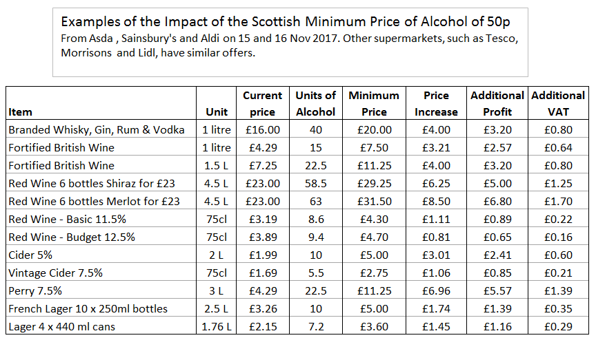
This week the British Supreme Court cleared the way for the Alcohol (Minimum Pricing) (Scotland) Act 2012 to be enacted. The Scotch Whisky Association (SWA) had mounted a legal challenge to try to halt the price hike, which it said was disproportionate’ and illegal under European law. (Daily Mail) The Act will mandate that retailers have to charge a minimum of 50p per unit of alcohol. This will only affect the price of alcohol in off-licences and supermarkets. In the pub, the price of a pint with 5% ABV is already much higher than the implied price of £1.42. I went round three supermarkets – Asda, Sainsbury’s and Aldi – to see the biggest price hikes implied in the rise.

The extra profit is kept by the retailer, though gross profits may fall as sales volume falls. Premium brands only fall below the minimum price in promotions. With the exception of discounter Aldi, the vast majority of shelf space is occupied by alcohol above the minimum price. Further, there is no escalator. The minimum price will stay the same for the six years that the legislation is in place. However, the Scottish Government claims that 51% of alcohol sold in off-trade is less than 50 pence per unit. The promotions have a big impact. The Scottish people will be deprived of these offers. Many will travel across the border to places like Carlisle and Berwick, to acquire their cheap booze. Or enterprising folks will break the law by illegal sales. This could make booze more accessible to underage drinkers and bring them into regular contact with petty criminals. However, will it reduce the demand for booze? The Scottish Government website quotes Health Secretary Shona Robison.

“This is a historic and far-reaching judgment and a landmark moment in our ambition to turn around Scotland’s troubled relationship with alcohol.

“In a ruling of global significance, the UK Supreme Court has unanimously backed our pioneering and life-saving alcohol pricing policy.

“This has been a long journey and in the five years since the Act was passed, alcohol related deaths in Scotland have increased. With alcohol available for sale at just 18 pence a unit, that death toll remains unacceptably high.

“Given the clear and proven link between consumption and harm, minimum pricing is the most effective and efficient way to tackle the cheap, high strength alcohol that causes so much damage to so many families.

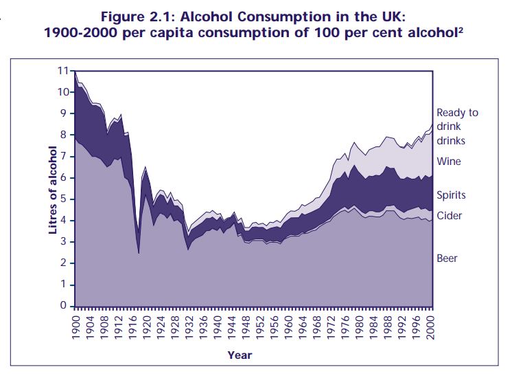
Is minimum pricing effective? Clearly, it will make some alcohol more expensive. But it must be remembered that the tax on alcohol is already very high. The cheapest booze on my list, per unit of alcohol, is the 3 litre box of Perry (Pear Cider) at £4.29. The excise duty is £40.38 per hectolitre. With VAT at 20%, tax is £1.92, or 45% of the retail price. The £16 bottles of spirits (including two well-known brands of Scottish Whisky) are at 40% alcohol. With excise duty at £28.74 per litre of pure alcohol, tax is £13.33 or 83% of the retail price. It has been well-known that alcohol is highly inelastic with respect to price so very large increases in price will make very little difference to demand. This is born out by a graphic from a 2004 report Alcohol Harm Reduction Strategy for England of the UK alcohol consumption in the last century.

In the early part of the twentieth century, there was sharp fall in alcohol consumption from 1900 to the 1930s. There was a sharp drop in the First World War, but after the war the decline continued the pre-war trend. This coincided with a religious revival and the temperance movement. It was started in the nineteenth century by organisations such as the Salvation Army and the Methodists, but taken up by other Christian denominations. In other words, it was a massive cultural change from the bottom, where it became socially unacceptable for many even to touch alcohol. Conversely, the steep decline in religion in the post-war period was accompanied by the rise in alcohol consumption.

The minimum price for alcohol is a fiscal solution being proposed for cultural problems. The outcome of a minimum price will be monopoly profits for the supermarkets and the manufacturers of alcoholic drinks.

It is true that a lot of crime is committed by those intoxicated, other social problems are caused and there are health issues. But the solution is not to increase the price of alcohol. The solution is to change people. The Revival of the early twentieth century, (begun before the outbreak of the Great War in 1914) saw both a fall in alcohol consumption and a fall in crime levels, that continued through the Great Depression. But it was not lacking of alcohol that reduced crime on the early twentieth. Instead, both reductions had a common root in the Christian Faith.

The Scottish Government will no doubt see a fall in sales of alcohol. But this will not represent the reduction in consumption, as cheaper booze will be imported from England, including Scottish Whisky. All that they are doing is treating people as statistics to be dictated to, and manipulated by, their shallow moralistic notions.

Kevin Marshall


The Morning Star’s denial of the Venezuelan Dictatorship

Guido Fawkes has an excellent example of the hard left’s denial of realities that conflict with their beliefs. From the Daily Politics, this is Morning Star editor Ben Chacko saying that the UN Human Rights Watch report on Venezuela was one-sided.

The Human Rights report can be found here.

The recent demonstrations need to be put into context. There are two contexts that can be drawn upon. The Socialist Side (with which many Socialists will disagree) is from Morning Star’s piece of 25th August The Bolivarian Revolution hangs in the balance.

They say

One of the world’s largest producers of oil, on which 95 per cent of its economy depends, the Bolivarian socialist government of Venezuela has, over the last 17 years, used its oil revenues to cut poverty by half and reduce extreme poverty to 5.4 per cent.

The government has built social housing; boosted literacy; provided free healthcare and free education from primary school to universities and introduced arts, music and cultural analysis programmes and many others targeting specific problems at the local level.

This is sentance emphasises the hard-left bias.

The mainly middle-class protesters, most without jobs and income, accused President Nicolas Maduro of dictatorship and continued with their daily demonstrations and demands for a change of government. 

Folks without “jobs or income” are hardly middle-class, but might be former middle-class. They have been laid low by circumstances. Should they be blaming the Government or forces outside the Government’s control?


From Capx.co on 16th August – Socialism – not oil prices – is to blame for Venezuela’s woes. Also from upi.com on 17th February – Venezuela: 75% of the population lost 19 pounds amid crisis. This is the classic tale of socialism’s failure.

  • Government control of food supplies leads to shortages, which leads to rationing, which leads to more shortages and black market profiteering. This started in 2007 when oil prices were high, but not yet at the record high.
  • Inflation is rampant, potentially rising from 720% in 2016 to 1600% this year. This is one of the highest rates in the world.
  • The weight loss is due to food shortages. It is the poorest who suffer the most, though most of the population are in extreme poverty.
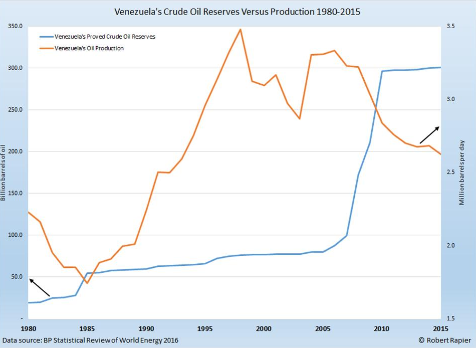
  • An oil-based economy needs to diversify. Venezuela has not. It needs to use high oil prices to invest in infrastructure. Instead, the Chavez regime expropriated the oil production from successful private companies and handed to Government Cronies. A graphic from Forbes illustrates the problem.

About a decade ago at the height of the oil price boom, Venezuela’s known oil reserves more than tripled, yet production fell. It now has the highest oil reserves of any country in the world.

  • Crime has soared, whilst people are going hungry.
  • Maybe a million children are missing school through hunger and lack of resources to run schools. Short-run “successes” based on expropriating the wealth of others have reversed to create a situation far worse than before Chavez came to power.
  • Oil prices are in real terms above the level they were from 1986 to 2003 (with the exception of a peak for the first Gulf War) and comparable to the peak reached in 1973 with the setting up of the OPEC Cartel and oil embargo.

The reality is that Socialism always fails. But there is always a hardcore always in denial, always coming up with empty excuses for failure, often blaming it on others. With the rise of Jeremy Corbyn (who receives a copy of the Morning Star daily), this hardcore has have taken over the Labour Party. The example of Venezuela indicates the long-term consequences of their attaining power.

Kevin Marshall

Britain Stronger in Europe Letter

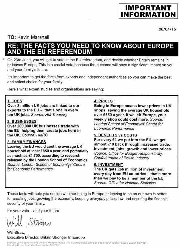
I received a campaign letter from Britain Stronger in Europe today headed

RE: THE FACTS YOU NEED TO KNOW ABOUT EUROPE AND THE EU REFERENDUM

Putting the “RE:” in front is a bit presumptuous. It is not a reply to my request. However, I believe in looking at both sides of the argument, so here is my analysis. First the main points in the body of the letter:-

  1. JOBS – Over 3 million UK jobs are linked to our exports to the EU.
  2. BUSINESSES – Over 200,000 UK Businesses trade with the EU, helping them create jobs in the UK.
  3. FAMILY FINANCES – Leaving the EU will cost the average UK household at least £850 a year, and potentially as much as £1,700, according to research released by the London School of Economics.
  4. PRICES – Being in Europe means lower prices in UK shops, saving the average UK household over £350 a year. If we left Europe, your weekly shop would cost more.
  5. BENEFITS vs COSTS – For every £1 we put into the EU, we get almost £10 back through increased trade, investment, jobs, growth and lower prices.
  6. INVESTMENT – The UK gets £66 million of investment every day from EU countries – that’s more than we pay to be a member of the EU.

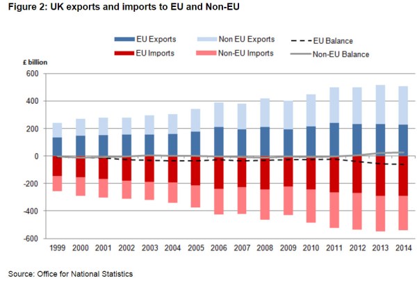
The first two points are facts, but only show part of the picture. The UK not only exports to the EU, but also imports. Indeed there is a net deficit with the EU, and a large deficit in goods. It is only due to a net surplus in services – mostly in financial services based in the City of London – that the trade deficit is not larger. The ONS provides a useful graphic illustrating both the declining share of exports to the EU, and the increasing deficit, reproduced below.

No one in the UK is suggesting that Brexit would mean a decline in trade, and it would be counter-productive for the EU not to reach a trade agreement with an independent UK when the EU has this large surplus.

The impact on FAMILY FINANCES is based upon the Centre for Economic Performance, an LSE affiliated organisation. There is both a general paper and a technical paper to back up the claims. They are modelled estimates of the future, not facts. The modelled costs assume Britain exits the European Union without any trade agreements, despite this being in the economic interests of both the UK and the EU. The report also does a slight of hand in estimating the contributions the UK will make post Brexit. From page 18 the technical paper

We assume that the UK would keep contributing 83% of the current per capita contribution as Norway does in order to remain in the single market (House of Commons, 2013). This leads to a fiscal saving of about 0.09%.

The table at the foot of report page 22 (pdf page 28) gives the breakdown of the estimate from 2011 figures. The Norway figures are gross and have a fixed cost element. The UK economy is about six times that of Norway, so would not end up spending nearly as much per capita even on the same basis. The UK figures are also a net figure. The UK pays into the EU twice as much as it gets out. Ever since joining the Common Market in 1973 Britain has been the biggest loser in terms of net contributions, despite the rebates that Mrs Thatcher secured with much effort in the 1980s.

The source of the PRICES information is again from the Centre for Economic Performance, but again with no direct reference. I assume it is from the same report, and forms part of the modelled forecast costs.

The BENEFITS vs COSTS statement is not comparing like with like. The alleged benefits to the UK are not all due to being a member of a club, but as a consequence of being an open economy trading with its neighbours. A true BENEFITS vs COSTS comparison would be future scenarios of Brexit vs Remain. Leading economist Patrick Minford has published a paper for the Institute of Economic Affairs, who finds there is a net benefit in leaving, particularly when likely future economic growth is taken into account.

The INVESTMENT issue is just part of the BENEFITS vs COSTS statement. So, like with the PRICES statement it is making one point into two.

 In summary, Britain Stronger in Europe claims I need to know six facts relevant to the referendum decision, but actually fails to provide a one. The actual facts are not solely due to the UK being a member of the European Union, whilst the relevant statements are opinions on modelled future scenarios that are unlikely to happen. The choice is between a various possible future scenarios in the European Union and possible future scenarios outside. The case for remain should be proclaiming the achievements of the European Union in making a positive difference to the lives of the 500 million people in the 28 States, along with future pathways where it will build on these achievements. The utter lack of these arguments, in my opinion, is the strongest argument for voting to leave.

Kevin Marshall


Copy of letter from Britain Stronger in Europe

Freeman Dyson on Climate Models

One of the leading physicists on the planet, Freeman Dyson, has given a video interview to the Vancouver Sun. Whilst the paper emphasizes Dyson’s statements about the impact of more CO2 greening the Earth, there is something more fundamental that can be gleaned.

Referring to a friend who constructed the first climate models, Dyson says at about 10.45

These climate models are excellent tools for understanding climate, but that they are very bad tools for predicting climate. The reason is simple – that they are models which have very few of the factors that may be important, so you can vary one thing at a time ……. to see what happens – particularly carbon dioxide. But there are a whole lot of things that they leave out. ….. The real world is far more complicated than the models.

I believe that Climate Science has lost sight of what this understanding of what their climate models actually are literally attempts to understand the real world, but are not the real world at all. It reminds me of something another physicist spoke about fifty years ago. Richard Feynman, a contemporary that Dyson got to know well in the late 1940s and early 1950s said of theories:-

You cannot prove a vague theory wrong. If the guess that you make is poorly expressed and the method you have for computing the consequences is a little vague then ….. you see that the theory is good as it can’t be proved wrong. If the process of computing the consequences is indefinite, then with a little skill any experimental result can be made to look like an expected consequence.

Complex mathematical models suffer from this vagueness in abundance. When I see supporters of climate arguing the critics of the models are wrong by stating some simple model, and using selective data they are doing what lesser scientists and pseudo-scientists have been doing for decades. How do you confront this problem? Climate is hugely complex, so simple models will always fail on the predictive front. However, unlike Dyson I do not think that all is lost. The climate models have had a very bad track record due to climatologists not being able to relate their models to the real world. There are a number of ways they could do this. A good starting point is to learn from others. Climatologists could draw upon the insights from varied sources. With respect to the complexity of the subject matter, the lack of detailed, accurate data and the problems of prediction, climate science has much in common with economics. There are insights that can be drawn on prediction. One of the first empirical methodologists was the preeminent (or notorious) economist of the late twentieth century – Milton Friedman. Even without his monetarism and free-market economics, he would be known for his 1953 Essay “The Methodology of Positive Economics”. Whilst not agreeing with the entirety of the views expressed (there is no satisfactory methodology of economics) Friedman does lay emphasis on making simple, precise and bold predictions. It is the exact opposite of the Cook et al. survey which claims a 97% consensus on climate, implying that it relates to a massive and strong relationship between greenhouse gases and catastrophic global warming when in fact it relates to circumstantial evidence for a minimal belief in (or assumption of) the most trivial form of human-caused global warming. In relation to climate science, Friedman would say that it does not matter about consistency with the basic physics, nor how elegantly the physics is stated. It could be you believe that the cause of warming comes from the hot air produced by the political classes. What matters that you make bold predictions based on the models that despite being simple and improbable to the non-expert, nevertheless turn out to be true. However, where bold predictions have been made that appear to be improbable (such as worsening hurricanes after Katrina or the effective disappearance of Arctic Sea ice in late 2013) they have turned out to be false.

Climatologists could also draw upon another insight, held by Friedman, but first clearly stated by John Neville Keynes (father of John Maynard Keynes). That is on the need to clearly distinguish between the positive (what is) and the normative (what ought to be). But that distinction was alienate the funders and political hangers-on. It would also mean a clear split of the science and policy.

Hattips to Hilary Ostrov, Bishop Hill, and Watts up with that.


Kevin Marshall

DECC’s Dumb Global Calculator Model

On the 28th January 2015, the DECC launched a new policy emissions tool, so everyone can design policies to save the world from dangerous climate change. I thought I would try it out. By simply changing the parameters one-by-one, I found that the model is both massively over-sensitive to small changes in input parameters and is based on British data. From the model, it is possible to entirely eliminate CO2 emissions by 2100 by a combination of three things – reducing the percentage travel in urban areas by car from 43% to 29%; reducing the average size of homes to 95m2 from 110m2 today; and for everyone to go vegetarian.

The DECC website says

Cutting carbon emissions to limit global temperatures to a 2°C rise can be achieved while improving living standards, a new online tool shows.

The world can eat well, travel more, live in more comfortable homes, and meet international carbon reduction commitments according to the Global Calculator tool, a project led by the UK’s Department of Energy and Climate Change and co-funded by Climate-KIC.

Built in collaboration with a number of international organisations from US, China, India and Europe, the calculator is an interactive tool for businesses, NGOs and governments to consider the options for cutting carbon emissions and the trade-offs for energy and land use to 2050.

Energy and Climate Change Secretary Edward Davey said:

“For the first time this Global Calculator shows that everyone in the world can prosper while limiting global temperature rises to 2°C, preventing the most serious impacts of climate change.

“Yet the calculator is also very clear that we must act now to change how we use and generate energy and how we use our land if we are going to achieve this green growth.

“The UK is leading on climate change both at home and abroad. Britain’s global calculator can help the world’s crucial climate debate this year. Along with the many country-based 2050 calculators we pioneered, we are working hard to demonstrate to the global family that climate action benefits people.”

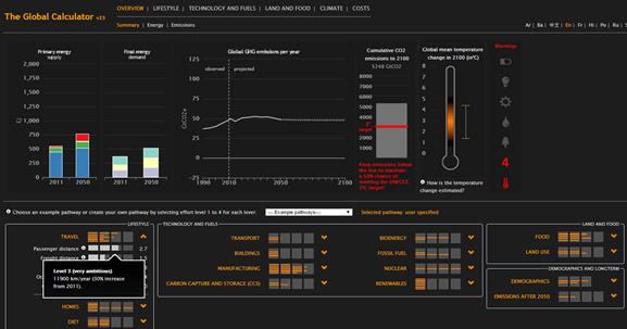
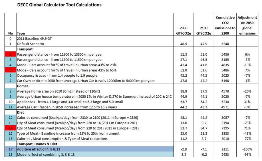
Upon entering the calculator I was presented with some default settings. Starting from a baseline emissions in 2011 of 49.9 GT/CO2e, this would give predicted emissions of 48.5 GT/CO2e in 2050 and 47.9 GT/CO2e in 2100 – virtually unchanged. Cumulative emissions to 2100 would be 5248 GT/CO2e, compared with 3010 GT/CO2e target to give a 50% chance of limiting warming to a 2°C rise. So the game is on to save the world.

I only dealt with the TRAVEL, HOMES and DIET sections on the left.

I went through each of the parameters, noting the results and then resetting back to the baseline.

The TRAVEL section seems to be based on British data, and concentrated on urban people. Extrapolating for the rest of the world seems a bit of a stretch, particularly when over 80% of the world is poorer. I was struck first by changing the mode of travel. If car usage in urban areas fell from 43% to 29%, global emissions from all sources in 2050 would be 13% lower. If car usage in urban areas increased from 43% to 65%, global emissions from all sources in 2050 would be 7% higher. The proportions are wrong (-14% gives -13%, but +22% gives +7%) along with urban travel being too high a proportion of global emissions.

The HOMES section has similar anomalies. Reducing the average home area by 2050 to 95m2 from 110m2 today reduces total global emissions in 2050 by 20%. Independently decreasing average urban house temperature in 2050 from 17oC in Winter & 27oC in Summer, instead of 20oC & 24oC reduces total global emissions in 2050 by 7%. Both seem to be based on British-based data, and highly implausible in a global context.

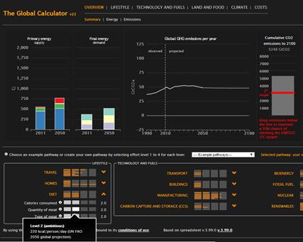
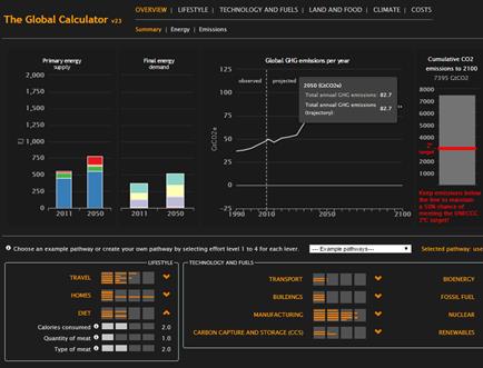
In the DIET section things get really silly. Cutting the average calorie consumption globally by 10% reduces total global emissions in 2050 by 7%. I never realised that saving the planet required some literal belt tightening. Then we move onto meat consumption. The baseline for 2050 is 220 Kcal per person per day, against the current European average of 281 Kcal. Reducing that to 14 Kcal reduces global emissions from all sources in 2050 by 73%. Alternatively, plugging in the “worst case” 281 Kcal, increases global emissions from all sources in 2050 by 71%. That is, if the world becomes as carnivorous in 2050 as the average European in 2011, global emissions from all sources at 82.7 GT/CO2e will be over six times higher the 13.0 GT/CO2e. For comparison, OECD and Chinese emissions from fossil fuels in 2013 were respectively 10.7 and 10.0 GT/CO2e. It seems it will be nut cutlets all round at the climate talks in Paris later this year. No need for China, India and Germany to scrap all their shiny new coal-fired power stations.

Below is the before and after of the increase in meat consumption.

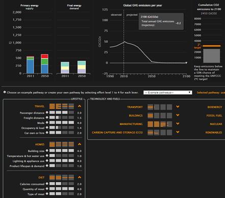
Things get really interesting if I take the three most sensitive, yet independent, scenarios together. That is, reducing urban car use from 43% to 29% of journeys in 2050; reducing the average home area by 2050 to 95m2 from 110m2; and effectively making a sirloin steak (medium rare) and venison in redcurrant sauce things of the past. Adding them together gives global emissions of -2.8 GT/CO2e in 2050 and -7.1 GT/CO2e in 2100, with cumulative emissions to 2100 of 2111 GT/CO2e. The model does have some combination effect. It gives global emissions of 3.2 GT/CO2e in 2050 and -0.2 GT/CO2e in 2100, with cumulative emissions to 2100 of 2453 GT/CO2e. Below is the screenshot of the combined elements, along with a full table of my results.

It might be great to laugh at the DECC for not sense-checking the outputs of its glitzy bit of software. But it concerns me that it is more than likely the same people who are responsible for this nonsense are also responsible for the glossy plans to cut Britain’s emissions by 80% by 2050 without destroying hundreds of thousands of jobs; eviscerating the countryside; and reducing living standards, especially of the poor. Independent and critical review and audit of DECC output is long overdue.

Kevin Marshall


A spreadsheet model is also available, but I used the online tool, with its’ excellent graphics. The calculator is built by a number of organisations.

Spending Money on Foreign Aid instead of Renewables

On the Discussion at BishopHill, commentator Raff asked people whether the $1.7 trillion spent so far on renewables should have been spent on foreign aid instead. This is an extended version of my reply.

The money spent on renewables has been net harmful by any measure. It has not only failed to even dent global emissions growth, it will also fail even if the elusive global agreement is reached as the country targets do not stack up. So the people of the emissions-reducing countries will bear both the cost of those policies and practically all the costs of the unabated warming as well. The costs of those policies have been well above anything justified in the likes of the Stern Review. There are plenty of British examples at Bishop Hill of costs being higher than expected and (often) solutions being much less effective than planned from Wind, solar, CCS, power transmission, domestic energy saving etc. Consequences have been to create a new category of poverty and make our energy supplies less secure. In Spain the squandering of money has been proportionately greater and likely made a significant impact of the severity of the economic depression.1

The initial justification for foreign aid came out of the Harrod and Domar growth models. Lack of economic growth was due to lack of investment, and poor countries cannot get finance for that necessary investment. Foreign Aid, by bridging the “financing gap“, would create the desired rate of economic growth. William Easterly looked at 40 years of data in his 2002 book “The Elusive Quest for Growth“. Out of over 80 countries, he could find just one – Tunisia – where foreign aid conformed to the theory. That is where increased aid was followed by increased investment which was followed by increased growth. There were plenty examples of where countries received huge amounts of aid relative to GDP over decades and their economies shrank. Easterly graphically confirmed what the late Peter Bauer said over thirty years ago – “Official aid is more likely to retard development than to promote it.

In both constraining CO2 emissions and Foreign Aid the evidence shows that the pursuit of these policies is not just useless, but possibly net harmful. An analogy could be made with a doctor who continues to pursue courses of treatment when the evidence shows that the treatment not only does not work, but has known and harmful side effects. In medicine it is accepted that new treatments should be rigorously tested, and results challenged, before being applied. But a challenge to that doctor’s opinion would be a challenge to his expert authority and moral integrity. In constraining CO2 emissions and promoting foreign aid it is even more so.

Notes

  1. The rationale behind this claim is explored in a separate posting.

Kevin Marshall