Last month the BBC headlined an article “Shell facing first UK legal claim over climate impacts of fossil fuels“. Typhoon Rai hit the Philippines in late 2021, damaging millions of homes and resulting in 400 deaths. Some of those affected are suing major oil producer Shell in UK courts, claiming that its emissions had a material impact on the severity of that typhoon. The BBC article states
The letter argues that Shell is responsible for 2% of historical global greenhouse gases, as calculated by the Carbon Majors database of oil and gas production, external.
The company has “materially contributed” to human driven climate change, the letter says, that made the Typhoon more likely and more severe.
The group wants to apply Philippine law (where the damage occurred) in a case to be heard in English courts. I will apply my rather cursory understanding of English tort law. That is, it is up to the litigant to prove their case on the balance of probabilities in an adversarial court system. A case is proved with clear evidence. In this case, each piece of evidence needs to be critically reviewed in light of the connection between human emissions and rising greenhouse gas levels; rising greenhouse gas levels and global average temperature rise; the rise in global average temperatures causing (or excerbating) Typhoon Rai; and the damage caused (especially injury and death being related to some function of (a) the strength of the storm and (b) the population impacted). Being a (somewhat) manic former beancounter, I will concentrate on the empirical data. I will also use a Greenpeace article from 23/10/25, which provides much more detail and a useful link to an attribution study.
That 2% figure
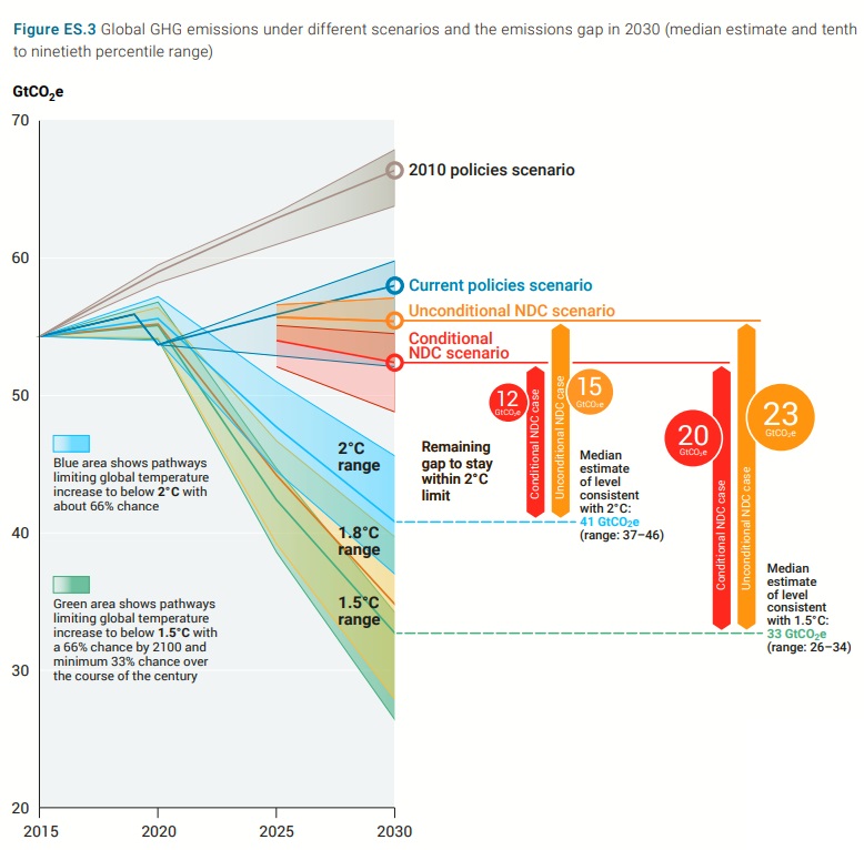
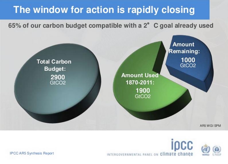
The BBC article states “that Shell is responsible for 2% of historical global greenhouse gases“. This is incorrect. The Greenpeace article gets closer, when it states “41 billion tons of CO2e or more than 2% of global fossil fuel emissions.” Going to the Carbon Majors Shell Page, the information box states that the 41.092 GtCO2 is 2.04% of the total CO2 emissions tracked by Carbon Majors from fossil fuels and cement for the period 1751-2013. This means that total emissions in the database were 2014 GtCO2.
Many would dispute whether a 2% contribution is a material contribution. There is a problem with this estimate. Anthropogenic CO2 emissions are mostly from fossil fuel emissions and cement production, but not entirely. There are also emissions from land-use changes. Further, I believe that the most authoritative source of anthropogenic CO2 emissions estimates are from the UNIPCC Assessment Reports. The most recent edition was the Sixth Assessment Report (AR6), published in 2021. AR6 WG3 SPM stated “Historical cumulative net CO2 emissions from 1850 to 2019 were 2400 ± 240 GtCO2 (high confidence)”. Footnote 10 states that this is at the 68% confidence interval. I was taught over 40 years ago that normal, acceptable, statistical confidence intervals were 95%, or double the 68% value. For a legal case in the UK, this should be confirmed by a Chartered Statistician (CStat) of the Royal Statistical Society (RSS), along with a validation of whether the confidence interval was calculated by a valid statistical method. AR6 used data from the Global Carbon Budget. AR6 is a bit coy about citing this source. However, searching “Friedlingstein” in the pdf of the full AR6 WG1 report, gives a reference to Friedlingstein et al., 2019. This is an annual, peer-reviewed article on the Global Carbon Budget.
The period 1850-2019 of the Global Carbon Budget is a century less than the Carbon Majors period of 1751-2023. To reconcile two data sets, I will ignore the period 1751-1849, as anthropogenic CO2 emissions were a tiny fraction of emissions since 1850. The Global Carbon Budget estimates CO2 emissions in 2019 at over 42 GtCO2, so the period 1850-2023 has emissions of 2570 ± (at least) 514 GtCO2. Ignoring the uncertainties, the Shell “share” of CO2 emissions becomes, at most, 1.6% of the total.
CO2 Emissions and Global Warming
However, this estimate ignores the impact of other greenhouse gas emissions on global warming. What about the impact of methane (CH4) emissions from bovine belching and flatulence? Or the methane emissions from sewage, or rotting waste? Or the Nitrous Oxide (N2O) emissions from burning heavy fuel oil in large container ships and supertankers?
The last IPCC assessment report attempted to attribute the observed relative global warming from 1850-1990 to 2010-2019 to various radiative forcing factors. The key graphic from AR6 WG1 SPM is reproduced as figure 1.
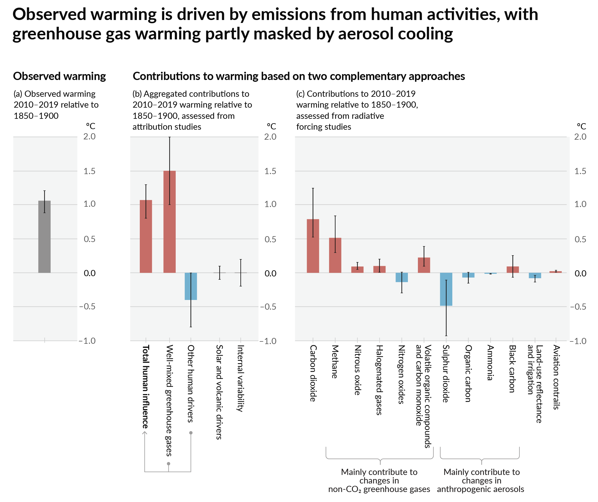
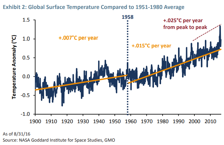
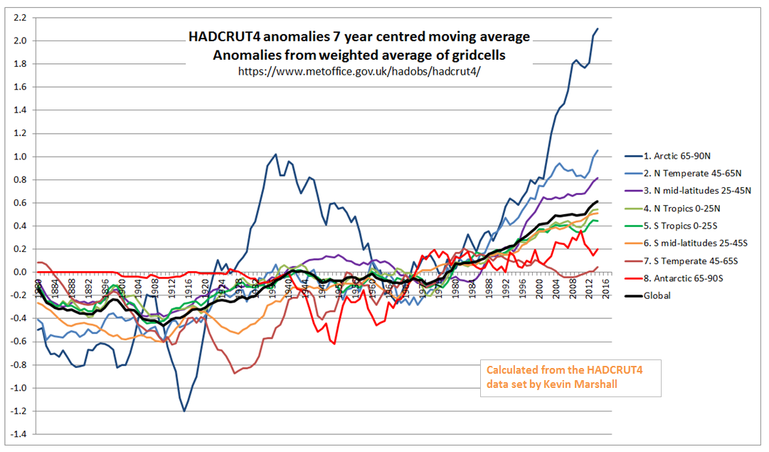
The key graphic is (c). Carbon dioxide emissions created about 0.8 °C of warming, of which around 80% was from the burning of fossil fuels. Adding to this are the methane emissions from the production of fossil fuels, along with the nitrous oxide and carbon monoxide emissions. Subtracting from this are emissions of nitrogen oxides and sulphur dioxide. The net impact is that about two-thirds of the observed warming. Pro rata, Shell is “responsible” for around 1% of the warming impact or about 0.01 °C of average global temperature over 150 years. Even this could very well be an exaggeration for two reasons. First, the calculated average temperature rise could be biased upwards. Second, some of the true average temperature rise could be due to natural factors, including variations caused by the chaotic nature of climate, or highly complex factors that are incapable of being described by scientific modelling. Much of the warming could be due to a rebound from a period called the Little Ice Age. Further, there was considerable warming during 1910-1940 in the data sets, which, a few years ago, was comparable in magnitude to the post-1975 warming. Yet the global emissions and the rate of rise in CO2 levels were considerably lower than in the later period.
Even using the data from the IPCC AR6, it is very difficult to establish, using a balance of probabilities criterion, that 41 GtCO2 of CO2 emissions raised global average temperatures by at least 0.01 °C since 1850-1900.
Impact of global warming on Typhoons in the Philippines
The BBC article grabbed my attention with the claim that human-caused emissions had made Typhoon Kai both more likely and severe. I am somewhat sceptical, as my cursory knowledge of the empirical evidence is that there is no convincing support for the hypothesis that tropical cyclones (typhoons in the eastern hemisphere, hurricanes in the western hemisphere) have increased markedly since the mid-70s when the rate of global average temperature rise took off. Such a correlation, if established, would be the starting point for claiming that the warming caused the increase.
There are two sources.
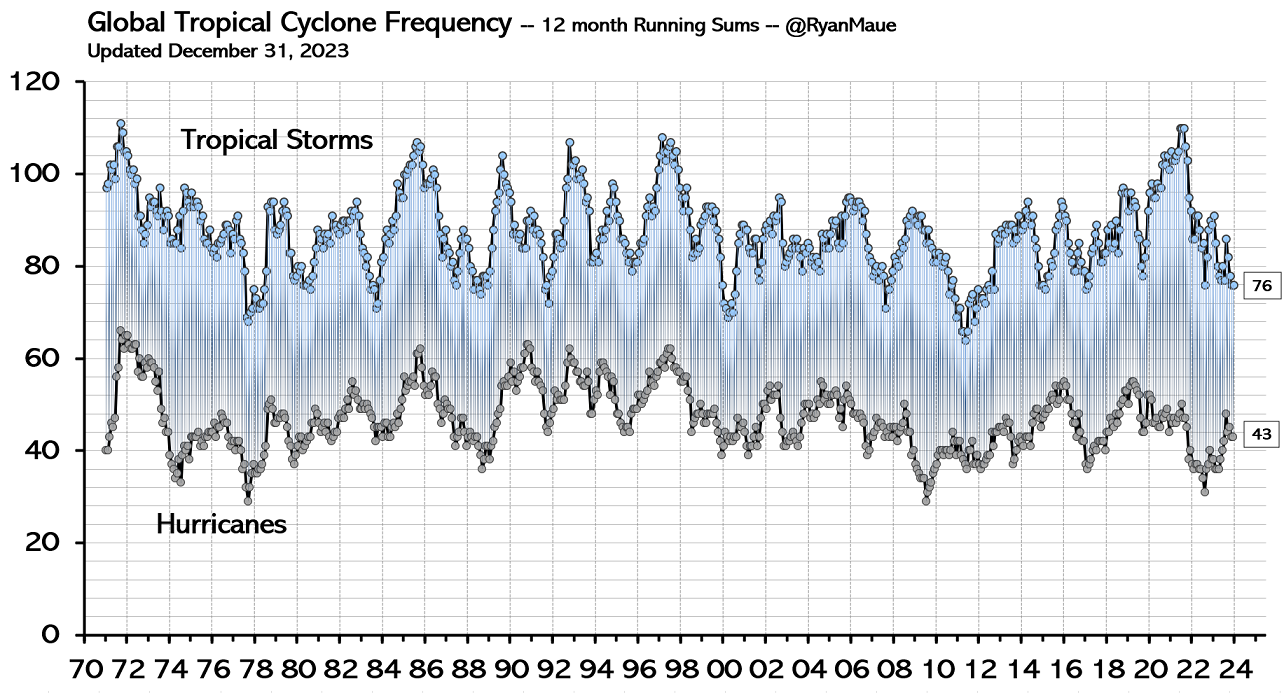
First is a couple of charts from Meteorologist Ryan Maue. These are of tropical cyclone frequency, and global tropical cyclone accumulated cyclone energy (from a peer-reviewed article). Both show data from the early 1970s. Cyclone frequency shows no trend. The cyclone frequency chart is more interesting. There are two major humps in the 1990s; a single peak in the 2000s; a relative energy drought 2008-2015; twin humps 2015-2020 smaller than the 1990s: then a decline into 2023 when the data ceases. At the foot of the chart there is a note. “Global data completeness much lower in the 1970s.” In terms of complete decades, the 1990s and 2000s seem tied for first, then the 2010s, with the 1980s in clear last place.
The second source has charts of Continental US hurricanes making landfall from Roger Pielke Jr. The big advantage is 125 years of consistent data, with no trend in all hurricanes or major hurricanes of Cat 3 and above. With this latest data is an accumulated cyclone energy chart for 1980-2024. This one has a single bar for each calendar year, with a slight downward trend.
With these data-driven prejudices, I took a look at the attribution study that supported the claim of human-caused climate change making Typhoon Rai more likely and more severe. This is, according to the Greenpeace Article, Clarke et al 2025 (The influence of anthropogenic climate change on Super Typhoon Odette (Typhoon Rai) and its impacts in the Philippines). The abstract states
First, we check that the current generation of higher resolution models used in attribution studies can capture the low sea level pressure anomaly associated with Typhoon Odette and hence can be used to study this type of event. A short analysis then compares such circulation analogues and the associated meteorological extremes over three time periods: past (1950-1970), contemporary (2001-2021), and future (2030-2050). Second, a multi-method multi-model probabilistic event attribution finds that extreme daily rainfall such as that observed during Typhoon Odette, has become about twice as likely
during the Typhoon season over the southern-central Philippines due to ACC. Third, a large ensemble tropical cyclone hazard model finds that the wind speeds of category 5 landfalling typhoons like Odette have become approximately 70% more likely due to ACC.
Viewing the data analysis and modelling as a black box, inputting data for 1950-1970 and 2001-2021 leads to the conclusion that Cat 5 Typhoon Odette (Rai) was made 70% more likely due to anthropogenic climate change (ACC). To ensure that this conclusion is not an artifact of inconsistent data quality, the processing of that data before inputting it into the models, and the modelling, one would need to see the complete set of raw data. As a preliminary, a count of each category of typhoon for each of the seven decades, or even by year. Why is this important? On a global level, Ryan Maue warned that global data completeness was much lower in the 1970s, which implies that it was improving. That improvement would have been most marked in the areas with the lowest completeness before the 1970s. The Philippines, a developing country made up of a many islands, probably had much poorer data quality in 1950-1970 than the continental USA. Yet Clarke et al is able, in Figure 1, to show maximum wind speeds as Odette/Rai tracked across the mid-Philippines. Data that could have only come from satellites. 60 years earlier, the calculation of typhoon strength could only have come from measurements on the ground, which may have been very few. Therefore, that raw data could often understate the typhoon category. And if there is no data for measured sub-Cat 1 typhoons, then the total number might be understated. Quite detailed data processing is therefore required to obtain approximately comparable data for the 1950s & 1960s with the 21st century. The less processing, the greater the chance of showing an increase that does not exist in reality, but the greater the processing, the greater the distance from actual data. Does Clarke et al tackle this issue?
Under 3.2.1 Observational data on page 18 is stated
In this section, we use a range of gridded observational and reanalysis products.
They haven’t even examined the real raw data. We can’t get any appreciation of how much the data has been transformed.
All is not lost for those who want to make a case for an ACC-caused increase in major typhoons in the Philippines. The UNIPCC has been struggling to make the connection for decades on a global basis. The 2021 AR6 WG1 (The Physical Science Basis) states in para A.3.4
It is likely that the global proportion of major (Category 3–5) tropical cyclone occurrence has increased over the last four decades, and it is very likely that the latitude where tropical cyclones in the western North Pacific reach their peak intensity has shifted northward; these changes cannot be explained by internal variability alone (medium confidence). There is low confidence in long-term (multi-decadal to centennial) trends in the frequency of all-category tropical cyclones. Event attribution studies and physical understanding indicate that human-induced climate change increases heavy precipitation
associated with tropical cyclones (high confidence), but data limitations inhibit clear detection of past trends on the global scale.
At the broadest level, my skeptical empiricist view is confirmed. There is no clear evidence of tropical cyclones having increased globally. Which means that the likely claim of major tropical cylones increasing is of a trivial quantity, or minor tropical cyclones have decreased. The significant part is about the western North Pacific. Given that there are a number of other areas globally where tropical cyclones occur, this is somewhat that this is the only area where an ACC influence can be found. But the Philippines could be construed as being in the western North Pacific, if the boundary between north and south is strictly the equator. The main islands of the Philippines lie 5 °- 19 ° N, and the Tropic of Cancer 23.6 ° N. For that reason alone, it is worth investigating.
The full report has quite a few mentions of this finding. on page 1747 is the following reference
Sun, J., D.Wang, X. Hu, Z. Ling, and L.Wang, 2019: Ongoing Poleward Migration of Tropical Cyclone Occurrence Over the Western North Pacific Ocean. Geophysical Research Letters, 46(15), 9110–9117,
doi:10.1029/2019gl084260.
Fortunately, the paper is open access. The Key Points are
- Tropical cyclone occurrence has been shifting poleward to the coast of East Asia from areas south of 20°N from 1982 to 2018
- The preferential tropical cyclone passage has switched from westward moving to northward recurving since 1998
- The poleward migration may be primarily attributed to the cyclonic anomaly of the steering flow over East Asia
The main point here is that south of 20°N (which the Philippines occupies), tropical cyclone occurrence has been decreasing. In case of doubt about the geography, check the colourful Figure 1. If one accepts the attribution to human-caused climate change, then the people of the Philippines should be thanking fossil fuel producers, not suing them. However, I am trying to look at what can be established on the balance of probabilities criterion. To repeat the comment in the WG1 SPM
….it is very likely that the latitude where tropical cyclones in the western North Pacific reach their peak intensity has shifted northward; these changes cannot be explained by internal variability alone (medium confidence).
In my (non-legal) opinion, there are two statements in this quotation.
The first is that there is evidence of climatic changes in the western North Pacific. The evidence is from statistical data (with potential data issues), but it far exceeds the balance of probabilities criterion.
The second is a qualitative opinion by a group of experts trying to find evidence of human-caused climate change. Medium confidence is tantamount to the opinion that, applying the balance of probabilities criterion, not even a small part of the observed change can be attributed to human causes.
Linking storm deaths to storm magnitude
In November 1970, Typhoon Bhola hit East Pakistan (now Bangladesh) and West Bengal. The official estimate was 500,000 dead. Most people were killed by the resulting storm surge that flooded the low-lying Ganges Delta. Another tropical cyclone hit Bangladesh in April 1991, killing at least 139,000. These are likely the first and third highest death tolls in the historical record for the old state of Bengal, although the further one goes back, the vaguer the reports. However, since 1991, the reporting of cyclones has become much more precise. The total deaths recorded in all cyclones by Wikipedia (which might be far from complete) since then are below 1,000. The likely reason for a greater than 99% fall in the deaths is the implementation of procedures to save lives. Like storm shelters and/or evacuation of the most vulnerable areas in advance of a cyclone. For the Philippines, with two-thirds of the population of Bangladesh, I count around 21,000 storm deaths in the period 2000-2025. This is highly skewed. The highest reported death toll was Typhoon Haiyan (Yolanda) in 2013 (6,352), followed by Tropical Storm Washi (Sendong) in 2011 (2,546) and Typhoon Bopha (Pablo) in 2012 (1,901). The three years 2011-2013 accounted for just over half the deaths in 2000-2025. The death rate per year from all storms 2000-2011 was about 3 times higher than in 2014-2025. Typhoon Kai in 2021, with 410 deaths, ranks ninth on the list. Of the deaths in 2014-2025, the two worst years were 2022 (467) and 2021 (463). Whilst the Philippines looks to have made great strides in reducing deaths from storms, there is clearly some way to go. That is if the Wikipedia figures are anything to go by.
Deaths are just one measure of the human impacts of powerful storms. There are also injuries, damage to property and the disruption to people’s lives. There has been much research on this topic in general, along with investigations afterwards to understand how the wide range of those human impacts can be lessened when similar events occur in the future. Whether or not the frequency of typhoons is increasing.
Conclusions and additional thoughts
Typhoon Rai was a Category 5 tropical cyclone that crossed the Philippines in December 2021, killing around 410 people. The claim has been made that the calculated 41 GtCO2 (2% of historical emissions) of CO2 emissions generated from the burning of fossil fuels extracted by Shell materially contributed to the severity of the storm.
The 2% material contribution is likely much smaller. In terms of the contribution to the human-caused global warming up to 2021, it is difficult to establish, through rigorous application of the balance probabilities criteria to AR6 WG1 evidence, that this quantity of emissions resulted in even 1% of the warming during 1850-2019. Even then, IPCC modelling makes the assumption that all the actual rise in global average temperatures is human-caused, which seems unwarranted when compared with the empirical evidence.
Key to attributing that warming to a 70% increase in the frequency of Cat 5 typhoons is data showing that such storms have increased both globally and in the Philippines area. The global data does not show such an increase. An attribution study comparing 1950-1970 and 2001-2021 did not look at the raw data. Thus, the authors cannot have looked at data quality and consistency issues in the entire period 1950-2021.
The attribution paper’s claimed increase in the frequency Cat 5 typhoons might conflict with the AR6 WG1 SPM report. The only case, the report finds, of climatic changes to global cyclones globally implies a reduction in tropical cyclones in the area of the Philippines during 1982-2018. Of course, it might still be that tropical cyclones were higher in 2001-2021 compared to 1950-1970, whilst declining during 1982-2018. But that still undermines the attribution paper.
Arguments about whether tropical cyclones have increased or not are invalid if the issue at stake is the human cost. A cursory look at the number of deaths suggests the death toll from the strongest typhoons appears to have decreased by over 90% since a run of severe storms in 2011-2013. This reduction is probably due to measures taken to reduce the human impacts.
As Shell has stated, the case against them is baseless. It is probably more baseless than they realised.
There are some additional thoughts on the Carbon Majors database. The most obvious one is why Shell. After all, BP is the largest historic British fossil fuel producer by potential emissions, although just 4% more than Shell. Globally, at the top of the list is China with seven times the “responsibility” of Shell. More generally, the database has three types of entities. These are (with shares) Investor-owned Company (24%), Nation State (15%) and State-owned Entity (30%). Smaller entities make up the remaining 31%. In fairness, any action should be a class-action suit against the whole world. That is not going to happen, so any successful action taken against investor-owned companies in, say UK or the USA, will be to the benefit of State entities in, say, China, Russia or Iran.
Kevin Marshall
Update 23rd April 2026
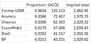
The Carbon Majors links are no longer valid. They were changed when the database was updated for 2024. The home page is https://carbonmajors.org/ and the list of entities is https://carbonmajors.org/Entities
The updated figures are below. If the figures and percentages are outputted from a single database, then dividing the GtCO2 figure by the percentage will give the same global total for emissions from fossil fuels. There is significant variation. For instance, the Aramco figure of 72.457 is 3.66% of 1980, or 3.51% of 2066.


