Summary
Following the publication of a survey finding a 97% consensus on global warming in the peer-reviewed literature the team at “skepticalscience.com” launched theconsensusproject.com website. Here I evaluate the claims using two of website owner John Cook’s own terms. First, that “genuine skeptics consider all the evidence in their search for the truth”. Second is that misinformation is highly damaging to democratic societies, and reducing its effects a difficult and complex challenge.
Applying these standards, I find that
- The 97% consensus paper is very weak evidence to back global warming. Stronger evidence, such as predictive skill and increasing refinement of the human-caused warming hypothesis, are entirely lacking.
- The claim that “warming is human caused” has been contradicted at the Sks website. Statements about catastrophic consequences are unsupported.
- The prediction of 8oF of warming this century without policy is contradicted by the UNIPCC reference.
- The prediction of 4oF of warming with policy fails to state this is contingent on successful implementation by all countires.
- The costs of unmitigated warming and the costs of policy and residual warming are from cherry-picking from two 2005 sources. Neither source makes the total claim. The claims of the Stern Review, and its critics, are ignored.
Overall, by his own standards, John Cook’s Consensus Project website is a source of extreme unskeptical misinformation.
Introduction
Last year, following the successful publication of their study on “Quantifying the consensus on anthropogenic global warming in the scientific literature“, the team at skepticalscience.com (Sks) created the spinoff website theconsensusproject.com.
I could set some standards of evaluation of my own. But the best way to evaluate this website is by Sks owner and leader, John Cook’s, own standards.
First, he has a rather odd definition of what skeptic. In an opinion piece in 2011 Cook stated:-
Genuine skeptics consider all the evidence in their search for the truth. Deniers, on the other hand, refuse to accept any evidence that conflicts with their pre-determined views.
This definition might be totally at odds with the world’s greatest dictionary in any language, but it is the standard Cook sets.
Also Cook co-wrote a short opinion pamphlet with Stephan Lewandowsky called The Debunking Handbook. It begins
It’s self-evident that democratic societies should base their decisions on accurate information. On many issues, however, misinformation can become entrenched in parts of the community, particularly when vested interests are involved. Reducing the influence of misinformation is a difficult and complex challenge.
Cook fully believes that accuracy is hugely important. Therefore we should see evidence great care in ensuring the accuracy of anything that he or his followers promote.
The Scientific Consensus
The first page is based on the paper
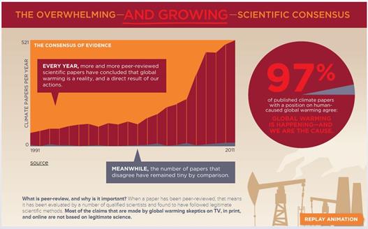
Cooks definition of a skeptic considering “all the evidence” is technically not breached. With over abstracts 12,000 papers evaluated it is a lot of evidence. The problem is nicely explained by Andrew Montford in the GWPF note “FRAUD, BIAS AND PUBLIC RELATIONS – The 97% ‘consensus’ and its critics“.
The formulation ‘that humans are causing global warming’ could have two different meanings. A ‘deep’ consensus reading would take it as all or most of the warming is caused by humans. A ‘shallow’ consensus reading would imply only that some unspecified proportion of the warming observed is attributable to mankind.
It is the shallow consensus that the paper followed, as found by a leaked email from John Cook that Montford quotes.
Okay, so we’ve ruled out a definition of AGW being ‘any amount of human influence’ or ‘more than 50% human influence’. We’re basically going with Ari’s porno approach (I probably should stop calling it that) which is AGW= ‘humans are causing global warming’. e.g. – no specific quantification which is the only way we can do it considering the breadth of papers we’re surveying.
There is another aspect. A similar methodology applied to social science papers produced in the USSR would probably produce an overwhelming consensus supporting the statement “communism is superior to capitalism”. Most papers would now be considered worthless.
There is another aspect is the quality of that evidence. Surveying the abstracts of peer-reviewed papers is a very roundabout way of taking an opinion poll. It is basically some people’s opinions of others implied opinions from short statements on tangentially related issues. In legal terms it is an extreme form of hearsay.
More important still is whether as a true “skeptic” all the evidence (or at least the most important parts) has been considered. Where is the actual evidence that humans cause significant warming? That is beyond the weak correlation between rising greenhouse gas levels and rising average temperatures. Where is the evidence that the huge numbers of climate scientists have understanding of their subject, demonstrated by track record of successful short predictions and increasing refinement of the human-caused warming hypothesis? Where is the evidence that they are true scientists following in the traditions of Newton, Einstein, Curie and Feynman, and not the followers of Comte, Marx and Freud? If John Cook is a true “skeptic”, and is presenting the most substantial evidence, then climate catastrophism is finished. But if Cook leaves out much better evidence then his survey is misinformation, undermining the case for necessary action.
Causes of global warming
The next page is headed.

There is no exclusion of other causes of the global warming since around 1800. But, with respect to the early twentieth century warming Dana Nuccitelli said
CO2 and the Sun played the largest roles in the early century warming, but other factors played a part as well.
However, there is no clear way of sorting out the contribution of the relative components. The statement “the causes of global warming are clear” is false.
On the same page there is this.

This is a series of truth statements about the full-blown catastrophic anthropogenic global warming hypothesis. Regardless of the strength of the evidence in support it is still a hypothesis. One could treat some scientific hypotheses as being essentially truth statements, such as that “smoking causes lung cancer” and “HIV causes AIDS”, as they are so very strongly-supported by the multiple lines of evidence1. There is no scientific evidence provided to substantiate the claim that global warming is harmful, just the shallow 97% consensus belief that humans cause some warming.
This core “global warming is harmful” statement is clear misinformation. It is extremely unskeptical, as it is arrived at by not considering any evidence.
Predictions and Policy
The final page is in three parts – warming prediction without policy; warming prediction with policy; and the benefits and costs of policy.
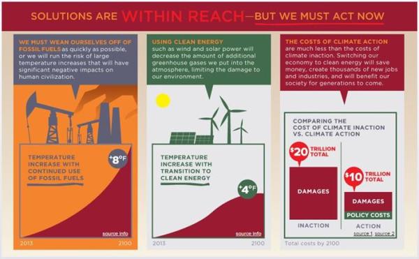
Warming prediction without policy
The source info for the prediction of 8oF (4.4oC) warming by 2100 without policy is from the 2007 UNIPCC AR4 report. It is now seven years out of date. The relevant table linked to is this:-
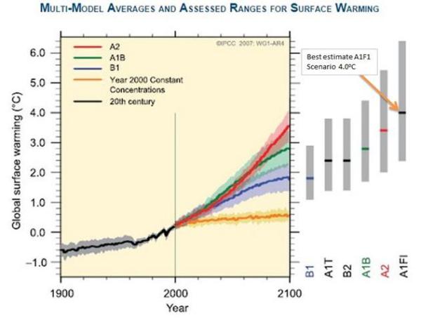
There are a whole range of estimates here, all with uncertainty bands. The highest has a best estimate of 4.0oC or 7.2oF. They seem to have taken the highest best estimate and rounded up. But this scenario is strictly for the temperature change at 2090-2099 relative to 1980-1999. This is for a 105 year period, against an 87 year period on the graph. Pro-rata the best estimate for A1F1 scenario is 3.3oC or 6oF.
But a genuine “skeptic” considers all the evidence, not cherry-picks the evidence which suit their arguments. If there is a best estimate to be chosen, which one of the various models should it be? In other areas of science, when faced with a number of models to use for future predictions the one chosen is the one that performs best. Leading climatologist, Dr Roy Spencer, has provided us with such a comparison. Last year he ran 73 of the latest climate CIMP5 models. Compared to actual data every single one was running too hot.
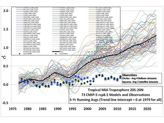
A best estimate on the basis of all the evidence would be somewhere between zero and 1.1oC, the lowest figure available from any of the climate models. To claim a higher figure than the best estimate of the most extreme of the models is not only dismissing reality, but denying the scientific consensus.
But maybe this hiatus in warming of the last 16-26 years is just an anomaly? There are at possibly 52 explanations of this hiatus, with more coming along all the time. However, given that they allow for natural factors and/or undermine the case for climate models accurately describing climate, the case for a single extreme prediction of warming to 2100 is further undermined. To maintain that 8oF of warming is – by Cook’s own definition – an extreme case of climate denial.
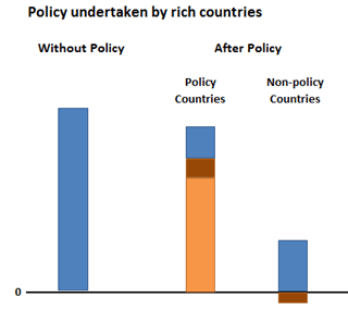
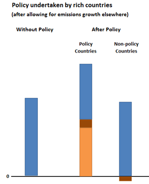
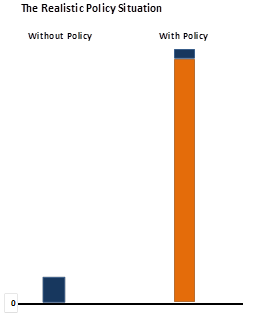
Warming prediction with policy
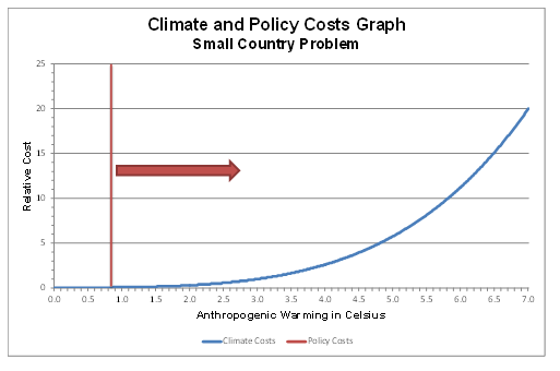
If the 8oF of predicted human-caused warming is extreme, then a policy that successfully halves that potential warming is not 4oF, but half of whatever the accurate prediction would be. But there are further problems. To be successful, that policy involves every major Government of developed countries reducing emissions by 80% (least including USA, Russia, EU, and Japan) by around 2050, and every other major country (at least including Russia, China, India, Brazil, South Africa, Indonesia and Ukraine) constraining emissions at current levels for ever. To get all countries to sign-up to such a policy combatting global warming over all other commitments is near impossible. Then take a look at the world map in 1925-1930 and see if you could reasonably have expected those Governments to have signed commitments binding on the Governments of 1945, let alone today. To omit policy considerations is an act of gross naivety, and clear misinformation.
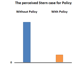
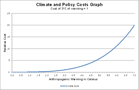
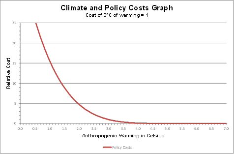
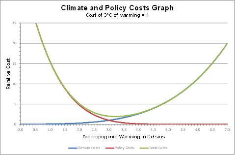
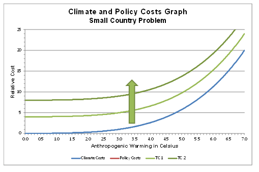
The benefits and costs of policy
The benefits and costs of policy is the realm of economics, not of climatology. Here Cook’s definition of skeptic does not apply. There is no consensus in economics. However, there are general principles that are applied, or at least were applied when I studied the subject in the 1980s.
- Modelled projections are contingent on assumptions, and are adjusted for new data.
- Any competent student must be aware of the latest developments in the field.
- Evaluation of competing theories is by comparing and contrasting.
- If you are referencing a paper in support of your arguments, at least check that it does just that.
The graphic claims that the “total costs by 2100” of action are $10 trillion, as against $20 trillion of inaction. The costs of action are made up of more limited damages costs. There are two sources for this claim, both from 2005. The first is from “The Impacts and Costs of Climate Change”, a report commissioned by the EU. In the Executive Summary is stated:-
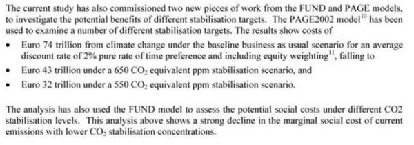
Given that €1.00 ≈ $1.20, the costs of inaction are $89 trillion and of reducing to 550ppm CO2 equivalent (the often quoted crucial level of 2-3 degrees of warming from a doubling of CO2 levels above pre-industrial levels) $38 trillion, the costs do not add up. However, the average of 43 and 32 is 37.5, or about half of 74. This gives the halving of total costs.
The second is from the German Institute for Economic Research. They state:-
If climate policy measures are not introduced, global climate change damages amounting to up to 20 trillion US dollars can be expected in the year 2100.
This gives the $20 trillion.
The costs of an active climate protection policy implemented today would reach globally around 430 billion US dollars in 2050 and around 3 trillion US dollars in 2100.
This gives the low policy costs of combatting global warming.
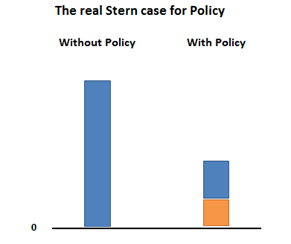
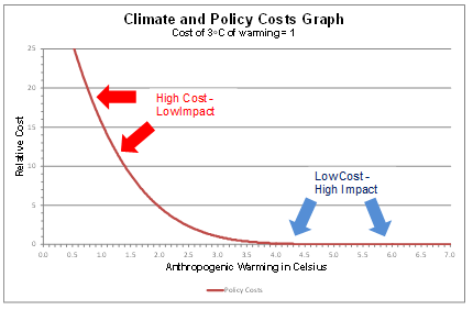
It is only by this arbitrary sampling of figures from the two papers that the websites figures can be established. But there is a problem in reconciling the two papers. The first paper has cumulative figures up to 2100. The shorthand for this is “total costs by 2100“. The $20 trillion figure is an estimate for the year 2100. The statement about the policy costs confirms this. This confusion leads the policy costs to be less than 0.1% of global output, instead of around 1% or more.
Further the figures are contradicted by the Stern Review of 2006, which was widely quoted in the UNIPCC AR4. In the summary of conclusions, Stern stated.
Using the results from formal economic models, the Review estimates that if we don’t act, the overall costs and risks of climate change will be equivalent to losing at least 5% of global GDP each year, now and forever. If a wider range of risks and impacts is taken into account, the estimates of damage could rise to 20% of GDP or more.
In contrast, the costs of action – reducing greenhouse gas emissions to avoid the worst impacts of climate change – can be limited to around 1% of global GDP each year.
The benefit/cost ratio is dramatically different. Tol and Yohe provided a criticism of Stern, showing he used the most extreme estimates available. A much fuller criticism is provided by Peter Lilley in 2012. The upshot is that even with a single prediction of the amount and effects of warming, there is a huge range of cost impacts. Cook is truly out of his depth when stating single outcomes. What is worse is that the costs and effectiveness of policy to greenhouse emissions is far greater than benefit-cost analyses allow.
Conclusion
To take all the evidence into account and to present the conclusions in a way that clearly presents the information available, are extremely high standards to adhere to. But theconsensusproject.com does not just fail to get close to these benchmarks, it does the opposite. It totally fails to consider all the evidence. Even the sources it cites are grossly misinterpreted. The conclusion that I draw is that the benchmarks that Cook and the skepticalscience.com team have set are just weapons to shut down opponents, leaving the field clear for their shallow, dogmatic and unsubstantiated beliefs.
Kevin Marshall
Notes
- The evidence for “smoking causes lung cancer” I discuss here. The evidence for “HIV causes AIDS” is very ably considered by the AIDS charity AVERT at this page. AVERT is an international HIV and AIDS charity, based in the UK, working to avert HIV and AIDS worldwide, through education, treatment and care. – See more here.
- Jose Duarte has examples here.