NOAA Future Aridity against Al Gore’s C20th Precipitation Graphic

Paul Homewood has taken a look at an article in yesterdays Daily Mail – A quarter of the world could become a DESERT if global warming increases by just 2ºC.

The article states

Aridity is a measure of the dryness of the land surface, obtained from combining precipitation and evaporation.  

‘Aridification would emerge over 20 to 30 per cent of the world’s land surface by the time the global temperature change reaches 2ºC (3.6ºF)’, said Dr Manoj Joshi from the University of East Anglia’s School of Environmental Sciences and one of the study’s co-authors.  

The research team studied projections from 27 global climate models and identified areas of the world where aridity will substantially change.  

The areas most affected areas are parts of South East Asia, Southern Europe, Southern Africa, Central America and Southern Australia.

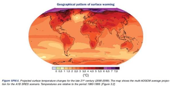
Now, having read Al Gore’s authoritative book An Inconvenient Truth there are statements first about extreme flooding, and then about aridity (pages 108-113). The reason for flooding coming first is on a graphic of twentieth-century changes in precipitation on pages 114 & 115.

This graphic shows that, overall, the amount of precipitation has increased globally in the last century by almost 20%.

 However, the effects of climate change on precipitation is not uniform. Precipitation in the 20th century increased overall, as expected with global warming, but in some regions precipitation actually decreased.

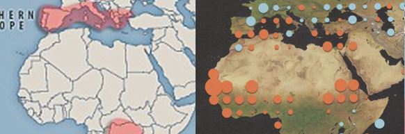
The blue dots mark the areas with increased precipitation, the orange dots with decreases. The larger the dot, the larger the change. So, according to Nobel Laureate Al Gore, increased precipitation should be the far more common than increased aridity. If all warming is attributed to human-caused climate change (as the book seems to imply) then over a third of the dangerous 2ºC occurred in the 20th century. Therefore there should be considerable coherence between the recent arid areas and future arid areas.

The Daily Mail reproduces a map from the UEA, showing the high-risk areas.

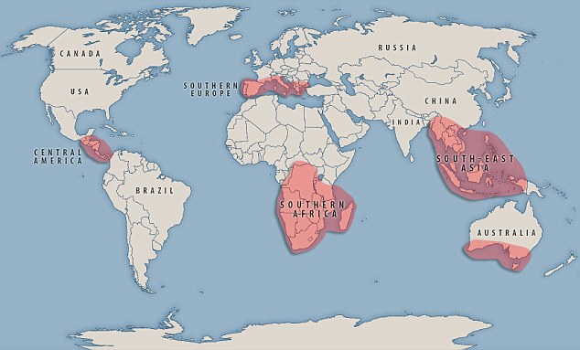
There are a couple of areas with big differences.

Southern Australia

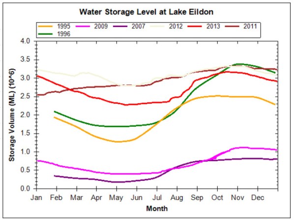
In the 20th century, much of Australia saw increased precipitation. Within the next two or three decades, the UEA projects it getting considerably arider. Could this change in forecast be the result of the extreme drought that broke in 2012 with extreme flooding? Certainly, the pictures of empty reservoirs taken a few years ago, alongside claims that they would never likely refill show the false predictions.

One such reservoir is Lake Eildon in Victoria. Below is a graphic of capacity levels in selected years. It is possible to compare other years by following the historical water levels for EILDON link.

Similarly, in the same post, I linked to a statement by re-insurer Munich Re stating increased forest fires in Southern Australia were due to human activity. Not by “anthropogenic climate change”, but by discarded fag ends, shards of glass and (most importantly) fires that were deliberately started.

Northern Africa

The UEA makes no claims about increased aridity in Northern Africa, particularly with respect to the Southern and Northern fringes of the Sahara. Increasing desertification of the Sahara used to be claimed as a major consequence of climate change. In the year following Al Gore’s movie and book, the UNIPCC produced its Fourth Climate Assessment Report. Working Group II report, Chapter 9 (Pg 448) on Africa made the following claim.

In other countries, additional risks that could be exacerbated by climate change include greater erosion, deficiencies in yields from rain-fed agriculture of up to 50% during the 2000-2020 period, and reductions in crop growth period (Agoumi, 2003).

Richard North took a detailed look at the background of this claim in 2010. The other African countries were Morocco, Algeria and Tunisia. Agoumi 2003 compiled three reports, only one of which – Morocco – had anything near a 50% claim. Yet Morocco seems, from Al Gore’s graphic to have had a modest increase in rainfall over the last century.

Conclusion

The UEA latest doom-laden prophesy of increased aridity flies in the face of the accepted wisdom that human-caused global warming will result in increased precipitation. In two major areas (Southern Australia and Northern Africa), increased aridity is at add odds with changes in precipitation claimed to have occurred in the 20th Century by Al Gore in An Inconvenient Truth. Yet over a third of the of the dangerous 2ºC warming limit occurred in the last century.

Kevin Marshall


Why Climate Change Mitigation Policies Will Always Fail

All climate mitigation policies will be of net harm to any country implementing them. There are three reasons for this.

First, mitigation policies will not eliminate all the projected harm of climate change. Policy replaces the unmitigated cost of climate change with a policy cost and a residual climate change cost.

Second, policy proposals are only for the rich countries to reduce emissions and emerging economies to constrain the growth. That means residual climate change costs will be greater, and the burden of cost of reductions will fall on a number of countries will a minority of, and a rapidly diminishing share of, global emissions. Even with the rich nations all succeeding in the British target of 80% reduction by 2050 will still mean global emission levels higher than currently.

Third, there is mounting evidence that actual mitigation costs per tonne of CO2 equivalent saved are considerably more than the economic models assume.


Introduction

The Stern Review Summary of Conclusions stated on page vi

Using the results from formal economic models, the Review estimates that if we don’t act, the overall costs and risks of climate change will be equivalent to losing at least 5% of global GDP each year, now and forever. If a wider range of risks and impacts is taken into account, the estimates of damage could rise to 20% of GDP or more.

In contrast, the costs of action – reducing greenhouse gas emissions to avoid the worst impacts of climate change – can be limited to around 1% of global GDP each year.

The Review further stated on pages xvi-xvii

Preliminary calculations adopting the approach to valuation taken in this Review suggest that the social cost of carbon today, is of the order of $85 per tonne of CO2……. This number is well above marginal abatement costs in many sectors.

Many objections to the report look at the cost of climate change. Little discussed are the theoretical issues in implementing a successful policy. By “successful” I mean where the expected outturn of the policy is less than the projected costs of climate change.


The basic case

As the Stern review is saying that globally we should replace one set of costs – the projected costs of climate change – will the much lesser costs of climate. Graphically, we replace the climate change costs in blue with policy costs in orange. Costs are positive and benefits negative.

The case for policy is clear.


Climate change costs not completely eliminated

Peter Lilley, in his 2012 GWPF report “WHAT IS WRONG WITH STERN?” states on page 8

The benefit of preventing (climate change) entirely would, on his figures, be at least 5% of GDP – but to do so would require not just stopping all further carbon emissions but removing all those accumulated since the industrial revolution. The action he proposes to reduce the worst impacts of global warming by stabilising the atmospheric concentration of greenhouse gases at 550 ppm would, using Stern’s methodology, save some 3.1% of GDP – not 5%.

The mitigation policy seeks to stabilize total greenhouse gas levels are a level equivalent to about double the level of CO2 in 1780.


The case for policy is still clear.


Rich Countries Policy Burden

It is accepted that

  1. Rich countries are responsible for most of climate change.
  2. The adverse consequences of unmitigated climate change will be disproportionately endured by the less developed nations (LDNs).

Therefore the moral argument is that the rich countries should bear the cost of policy and they should compensate the LDNs for the future harm that they will endure. The compensation could then be used to offset the harm of climate change.

Rich countries have a smaller population than the LDNs. The policy costs (in orange) for them will more than double. Similarly, compensation (in burnt orange) will be much larger for the rich countries to pay out than for the LDNs who receive it in income. Finally the post-policy climate change costs (in blue) will be still larger for the LDNs.


The rich countries may or may not be better off after policy. Further the LDNs still suffer some harm.


Increasing Emissions amongst the emerging nations

Policy must include the emerging nations. This is why.

I have arbitrarily split the countries of the World into three groups

  1. ACEJU – The big industrialised carbon emitters – Australia, Canada, EU, Japan and USA.
  2. BICS – The large emerging nations of Brazil, India, China and South Africa.
  3. ROW – Rest of the World.

The World Bank has data on CO2 emissions by country for the period 1990 to 2010. From this, I compiled the following graph.


In the period 1990 to 2010, annual global CO2 emissions increased by 11.4 billion tonnes, or 51%. To return to 1990 emissions levels would require one group to cease emissions entirely and the other two groups to maintain emissions at 2010 levels. The future emissions growth path potentially makes the problem worse. Consider the comparative growth in population.


Despite the BICS countries increasing its emissions by 230%, emissions per capita are still less than 40% of those of the ACEJU block. Further, the explosive growth of the BICS has not been matched by the Rest of the World. Here the emissions have grown by 45%, but population has grown by 42%. Emissions per capita are still only 35% of those of the AJEJU block.

Any policy reductions by the rich nations will be more than offset by future emissions growth in the rest of the world. There will be little reduction in climate change costs, for either the policy countries or non-policy countries. The situation becomes like this.


The non-policy countries will still see a reduction, but that might be small, even if the policy countries are successful. The disadvantage to the policy countries is inversely related to proportion of global emissions they have at the end of the policy. That in turn is influenced by the future emissions growth in the non-policy countries, as well as the proportion of global emissions in a baseline year.


Peer-reviewed costs of Climate Change and Actual Costs of Mitigation

The Stern review should not be taken as the only source. The UNIPCC AR4 Summary for Policymakers in 2007 stated on page 22.

Peer-reviewed estimates of the social cost of carbon in 2005 average US$12 per tonne of CO2, but the range from 100 estimates is large (-$3 to $95/tCO2).

The average social cost is just a seventh of the Stern Review, which was not a study that has been peer-reviewed.

In a previous posting, I calculated that the subsidy of offshore wind farms was equivalent to 3.8 times Stern’s social cost of carbon, and 27 times that of the $12 average of peer-reviewed studies quotes by the UNIPCC. This was a low estimate, not including transmission costs. There might be cheaper ways of abating CO2, but there are lot of failed policies as well. There is also the impact on economic growth to consider, which for emerging economies. So a more realistic situation of a “successful” mitigation policy will look like the one below. That is “successful” in achieving the emission reduction targets.

Points for further investigation

There are a number of issues that are raised in my mind that need further work.

  1. The social cost of carbon defines the expected harm from climate change per tonne of CO2. If a country has quantitative emissions reduction targets, then an absolute upper limit in annual spend can be defined when achieving that target.
  2. This would enable identification of the success of policies within a national plan, along with the overall success of that plan.
  3. The expected CO2 emissions growth in non-policy countries, along with including other greenhouse gas emissions within the analysis.


Conclusion

There is no combination of mitigation policies that can produce a less costly outcome than doing nothing. Any government unilaterally (or as part of group representing a minority of global emissions) pursuing such policies will be imposing net harm on its own people, no matter how large the claimed potential impacts of climate change. This conclusion can be reached even if the extreme views of the Stern Review are taken as the potential costs of climate change.

Kevin Marshall


Notes

The comparison of emissions growth between countries is derived from “The Climate Fix” by Roger Pielke Jnr. This enlarges on a comment made at Australian Climate Madness blog.

All first time comments are moderated. Please use the comments as a point of contact.

Update 25/02 17.30. Summary and “Points for further investigation” included, along with text changes

The Nub of the Climate Change Policy Problem

Over at the Conversation, Climate Scientist Mike Hulme has a short article “Science can’t settle what should be done about climate change“. He argues the politics, not science, must take centre stage. He makes four points.

  • How do we value future public goods and natural assets relative to their value today?
  • Is “commodifying” nature appropriate?
  • The morality of technologies for mitigation or adaptation. For instance, fracking and GM crops.
  • The role of national governments against multilateral treaties or international governing bodies. Also the consequent impacts on democracy.

Christopher Wright (Professor of Organisation Studies at University of Sydney) commented

The one problem I have with the above analysis is that the focus on climate science has been a quite deliberate strategy by those seeking to deny or cast doubt on the urgency of the problem. This has meant the debate has continually stalled around issues of whether climate change is a problem or not. The science highlights that it is a very big problem indeed. However, while the science continues to be questioned, we will be unable to have the serious policy conversation about what we need to do to avoid catastrophic changes to our ecosystem.

My reply (with references) is

Science might point to a very big problem, but it cannot translate that into coherent policy terms. Nor can it weigh that against the effectiveness of policies, nor the harms policies can cause. Economics is central to asking those questions. The key figure that encapsulates the predicted harm of climate change is the social cost of carbon SCC, expressed in tonnes of CO2 equivalent. In 2006 Stern measured this as $85/tCO21. A year later the AR4 SPM2 stated a range of -$3 to $95/tCO2 from peer reviewed studies, with an average of $12/tCO2.

The key figure for the effectiveness to policy is the marginal abatement cost. Basically this refers to the marginal cost of preventing a tonne of CO2 equivalent entering the atmosphere. For policy to be of net benefit, MAC needs to be less than SCC.

$85 is about £52, and $12 about £7.50. In the UK onshore wind turbines receive a direct subsidy equivalent to £98/tCO23 saved, and offshore £195/tCO2. Then there are the extra costs of transmission lines, and other costs which could double those figures.

Then you need to recognize that a global problem will not be solved by unilateralist policies by a country with producing less than 2% of global emissions. So the UK is impoverished now by harmful, ineffectual, policies, and still future generations suffer >90% of the consequences of unmitigated climate change. Mike Hulme’s four points above are in addition to this, weighing further against mitigation policy.

Notes

  1. The Stern review noted on pages xvi-xvii

    Preliminary calculations adopting the approach to valuation taken in this Review suggest that the social cost of carbon today, is of the order of $85 per tonne of CO2……. This number is well above marginal abatement costs in many sectors.

  2. The UNIPCC AR4 Summary for Policymakers in 2007 stated on page 22.

    Peer-reviewed estimates of the social cost of carbon in 2005 average US$12 per tonne of CO2, but the range from 100 estimates is large (-$3 to $95/tCO2).

  3. The renewables obligation credit (ROC) buy-out price is currently £42.02 per megawatt hour, as determined by OFGEM. The British renewable industry lobby group renewableUK, uses DECC’s carbon saving figure of 430g/kWh, as stated in an appendix to the Energy Efficiency Innovation Review in 2005. £42.02/.430 = £97.67. Onshore wind turbines get one ROC per MWh generated, offshore wind turbines 2 ROCs.

Kevin Marshall

Jo Nova discusses Mike Hulme’s four points here.

Radiative Forcing – UNIPCC AR5 undermines AR4, but scientists have unshaken confidence in their work

Last year in “Aerosols – The UNIPCC AR4 adjustment factor” I claimed that in 2007 the UNIPCC engineered the radiative forcing components to tell a story. It basically manipulated the figures to account for the lack of warming up to that point. The release of AR5 Working Group 1 report yesterday shows the extent of the false levels of certainty in the scientist’s estimates in 2007.

The Data

In 2007 Figure 2.4 of the Synthesis Report was as follows

In 2013, Figure SPM.5 is below1

There are slight changes in format and terminology. I have put the two tables side-by-side for comparison, with analysis:-


The range of forcings I have expressed the range as a percentage of the mid-point.

Below are comments on the individual forcing components.

Carbon Dioxide CO2

The most important anthropogenic greenhouse gas has hardly moved, from 1.66 to 1.68 W m-2. In 1750 CO2 levels were 280 ppm, rising to 379 ppm in 2005 and 392 ppm in 2011. In 2007, the scientists estimated that it took a rise of 60 ppm to increase radiative forcing by 1 W m-2, compared to 66 ppm in 2013. Scientists have found that CO2 is 10% less effective as a greenhouse gas than previously thought. They are far less certain about this figure, as the range has doubled, but they are still have high confidence in their figures4 but scientists have switched from high confidence to very high confidence with their figures.3

Methane CH4

CH4 has practically doubled in impact, from 0.48 to 0.97 W m-2. In 1750 CH4 levels were 715 ppb, rising to 1774 ppb in 2005 and 1803 ppb in 2011. In 2007, the scientists estimated that it took a rise of 2200 ppb to increase radiative forcing by 1 W m-2, compared to 1120 ppm in 2013. Scientists have found that CH4 was practically twice as potent as a greenhouse gas than previously thought. They are far less certain about this figure, as the range has more than doubled relative to the mid-point. More significantly, the new potency is well outside the confidence range of the 2007 report. There the high point of the uncertainty range was 0.53 W m-2, whereas the low point of the uncertainty range is 0.74 W m-2. Despite having been so far out six years ago the scientists still have high confidence in their figures. The reason given on page 9 is

This difference in estimates is caused by concentration changes in ozone and stratospheric water vapour due to CH4 emissions and other emissions indirectly affecting CH4.


The potency of CH4 is a modelled estimate based on other factors. It is by including these indirect effects that the uncertainty is increased.

As a side point, of the 1100 ppb rise in CH4 levels since 1750, 80% was prior to the 1975. It has ceased to be a significant contributor to increasing radiative forcing. Given the increased recognised potency, it is a minor explanation of the pause in warming.

Nitrous Oxide N2O

This has hardly moved in impact, from 0.16 to 0.17 W m-2. In 1750 N2O levels were 270 ppb, rising to 319 ppb in 2005 and 324 ppb in 2011. Scientists are far less certain about these figures, as the range has nearly doubled, but they still have high confidence in their figures.

Halocarbons4

Although a minor group of greenhouse gases the impact has reduced from 0.34 to 0.18 W m-2, but the magnitude to the uncertainty band has increased more than five-fold from 0.06 (0.37-0.31) to 0.34 (0.35-0.01). Instead of reducing scientists confidence, they have gone from “high confidence” to “very high confidence” in the figures.

Aerosols

Of the 2007 report I claimed they were a fudge factor, suppressing the warming effect of greenhouse gases. The combined mid-point is now 1.20 W m-2of direct and cloud albedo effects, down more than 30% on 2007. The range of uncertainty is more significant. This has increased from 0.8 to 0.9 W m-2, with the impact of the high-end being a net warming effect. Despite being now being uncertain of whether the direct effect of aerosols warm or cool the planet, and despite being less certain of already high “confidence” range six years ago, the scientists still have high confidence in their figures.

Forecasts for Radiative Forcing in 2100 for CO2 and CH4

Let us assume that CO2 continue to increase at 3ppm a year and CH4 increases by 5ppb a year until 2100. Using 2007 potency estimates, CO2 forcing will be 6.34 W m-2 and CH4 will be 0.69 W m-2 above 1750 levels. Using 2013 potency estimates, CO2 forcing will be 5.72 W m-2 and CH4 will be 1.37 W m-2 above 1750 levels. Combined estimated forcing is less than 1% different, despite doubling the potency of CH4. Maybe we will have a much greater reason to worry about the melting of permafrost in the tundra, causing a huge rise in atmospheric methane levels. Suppressed warming from this factor has been doubled.

Conclusion

Scientists now implicitly admit that they were much too confident about the potency of greenhouse gases in 2007. They have now doubled the uncertainty bands on the three major greenhouse gases. Yet recognizing this past over confidence seems to have had no impact on current levels of confidence.

Kevin Marshall


Notes

  1. The graphic at the time of writing was only available in pdf format.
  2. NMVOC = Non-methane volatile organic compounds. They have a role in the production of ozone. Defra have a fuller explanation.
  3. All these figures are available from the 2007 “Full report” page and the 2013 WG1 Summary for Policymakers page 7. This is the 27-09-13 version. Page numbering will change once tables are properly inserted.
  4. Upon re-reading I have made two adjustments. For CO2, I note that scientists have increased their confidence despite doubling the size of their uncertainty bands. I have also added a comment on halocarbons, where confidence has increased, despite a

Assessing the UNIPCC fifth assessment report

The first part of the UNIPCC AR5 is due to be published in the coming days. At the Conversation, Research Fellows Roger Jones and Celeste Young at Victoria University have posted Explainer: how to read an IPCC report. It contains some useful stuff on penetrating the coded language of the IPCC report. You will be better able to decode what the IPCC mean by various levels of confidence. However, the authors are very careful not to give people a free rein in thinking for themselves. Therefore they stress that the language is complex, and any questions need to be answered by an expert. After all, it would not do to have people misinterpreting the science.

I suggest an alternative method of understanding the science. That is comparing what is said now with what the consensus said back in 2007 in AR4. The AR4 is available at the United Nations Intergovernmental Panel on Climate Change website at the following location.

http://www.ipcc.ch/publications_and_data/publications_ipcc_fourth_assessment_report_synthesis_report.htm

Figure 2.4 Radiative forcing components of SYR.

It would be nice to see the comparative estimates, particularly on whether aerosols have a comparatively large negative role and whether natural factors are still less than 10% of the net total.

.

Figure 2.4. Global average radiative forcing (RF) in 2005 (best estimates and 5 to 95% uncertainty ranges) with respect to 1750 for CO2, CH4, N2O and other important agents and mechanisms, together with the typical geographical extent (spatial scale) of the forcing and the assessed level of scientific understanding (LOSU). Aerosols from explosive volcanic eruptions contribute an additional episodic cooling term for a few years following an eruption. The range for linear contrails does not include other possible effects of aviation on cloudiness. {WGI Figure SPM.2}

Figure SPM.6. Projected surface temperature changes for the late 21st century (2090-2099).

An updated map on a comparable basis would be useful, especially for the most concerning area of the Arctic.


Figure SPM.6. Projected surface temperature changes for the late 21st century (2090-2099). The map shows the multi-AOGCM average projection for the A1B SRES scenario. Temperatures are relative to the period 1980-1999. {Figure 3.2}

Table SPM.2. Examples of some projected regional impacts.


It would be nice to have an update on how the short term impacts are doing. These all had high confidence or very high confidence

In Africa

By 2020, between 75 and 250 million of people are projected to be exposed to increased water stress due to climate change.

By 2020, in some countries, yields from rain-fed agriculture could be reduced by up to 50%. Agricultural production, including access to food, in many African countries is projected to be severely compromised. This would further adversely affect food security and exacerbate malnutrition.

In Australia and New Zealand

By 2020, significant loss of biodiversity is projected to occur in some ecologically rich sites, including the Great Barrier Reef and Queensland Wet Tropics.

Small Islands

Sea level rise is expected to exacerbate inundation, storm surge, erosion and other coastal hazards, thus threatening vital infrastructure, settlements and facilities that support the livelihood of island communities.

Please note the graphs used are available at this website and are IPCC Copyright.


James Hansen favouring Richard Lindzen over IPCC

Much has been made of James Hansen’s recent claim in a youtube video that runaway global warming will make the oceans boil. However, people have not picked up an earlier point, where the father of global warming alarmism clearly contradicts the consensus.

In the first minute of the clip, Hansen talks about the impact of ice sheets disintegrating in the polar regions. All this extra cold fresh water decreases ocean temperatures. This, in turn, increases the temperature gradient between the poles and the tropics. This, in turn, increases the strength of storms.

If Hansen looks his own GISSTEMP figures for global average temperatures, he will notice that the warming has been higher is the Artic than in the tropics. According to UNIPCC in 2007, the fastest warming in this century will be in the Arctic. I propose that cooling of the Arctic Ocean will have two effects. First it will counterbalance the most extreme warming of the planet, thereby reduce the total temperature rise. Also it will counter-balance some of the rise in temperatures, so reducing the impact of Greenland ice melt and slowing the reduction in sea ice. Second, it will reduce the impact of extreme storms. If melting ice cools the oceans, it is a negative feedback.


Sources of the boiling oceans comment are:-

WUWT comments 2 and 3 by Eric Worrall

http://carbon-sense.com/ on April 13th 2013

C3 Headlines


Forcings – Hansen et al 2000 v UNIPCC 2007

Two months ago I did an analysis of aerosols in the UNIPCC AR4 report, observing that

  1. That the IPCC can’t add up.
  2. The figures appear contrived to show that only CO2 was the problem.

Anthony Watts has a posting today “Shocker: The Hansen/GISS team paper that says: “we argue that rapid warming in recent decades has been driven mainly by non-CO2 greenhouse gases“. This is based on the James Hansen (and others) paper analysing natural forcings, with the following graphic.


Hansen et al Figure 1: Estimated climate forcings between 1850 and 2000.

I thought that I would do a quick the comparison between what the IPCC were saying in 2007, with what Hansen et al. were saying in 2000.

According to the UNIPCC

  1. Hansen underestimated CO2 component.
  2. Hansen overestimated the CH4 component.
  3. Hansen overestimated the impact of the sun.

However, Hanson could counter that the UNIPCC have completely forgotten about the impact of volcanoes.

It could be completely coincidental, that further analysis by climate scientists gives a greater role to CO2, and therefore even stronger justification for constraining CO2 emissions. However, although they became more certain on positive forcings, they are less certain than Hansen on aerosols. It gives even greater credence to the cynical view that the climate science community are exaggerating the influence of anthropogenic forcings on climate. Given the billions of dollars annually being poured into research one could reasonably expect a reduction in the uncertainties over time.

Aerosols – The UNIPCC AR4 adjustment factor

Scientific effort should be dedicated towards resolving the biggest unknowns. After feedbacks, the largest area of uncertainty in forecasting future global warming is the measurement of radiative forcing components.

A quick analysis of the radiative forcing components table in the 2007 AR4 Summary Figure 2.4, page 17 (4.1MB pdf) , would suggest a number of fudge factors have been used to arrive at the results.

I have summarised the table below, less the fancy bars, but with the uncertainty spreads and some check totals.

Radiative Forcing Components
Derived from AR4 (accessed March 2012)

RF Effect (W m-2)

Forcing Component Mid-point

Low

High

Spread %

Carbon Dioxide

1.66

1.49

1.83

20%

Methane

0.48

0.43

0.53

21%

Nitrous Oxide

0.16

0.14

0.18

25%

Halocarbons

0.34

0.31

0.37

18%

Ozone – Stratospheric

-0.05

-0.15

0.05

400%

Ozone – Tropospheric

0.35

0.25

0.65

114%

Stratospheric water vapour from CH4

0.07

0.02

0.12

143%

Surface Albedo – Land Use

-0.20

-0.40

0.00

-200%

Surface Albedo – Black Carbon on Snow

0.10

0.00

0.20

200%

Aerosol – Direct effect

-0.50

-0.90

-0.10

-160%

Aerosol – Cloud lbedo effect

-0.70

-1.80

-0.30

-214%

Linear Contrails

0.01

0.003

0.03

270%

Net total

1.72

-0.61

3.56

242%

Of which:-
Positive Forcings

3.17

2.64

3.90

40%

Negative Forcings

-1.45

-3.25

-0.35

-200%

Assymetric Summing

1.72

0.65

2.29

96%

Total per the Report

1.60

0.60

2.40

113%

If these were financial figures, an external auditor might ask the following questions.

  1. Why do the columns not add up? The difference of 0.12 is the same as the figure for solar irradiance. I would guess that the error in the mid-point is due to someone having deducted this figure from the total, erroneously believing that they had previously included it.
  2. Given the breadth of uncertainty, is it more than a coincidence that the negative forcings almost exactly offset all the positive forcings with the exception of CO2? This conveniently reduces the language of the debate from discussing “anthropogenic greenhouse gases”, to “rising CO2”.
  3. Given the breadth of uncertainty, is it more than a coincidence that the range of negative forcings are exactly equal to 200% of the sum of the mid-points?
  4. Given the breadth of uncertainty, is it more than a coincidence that the range of postive forcings are almost exactly equal to 40% of the sum of the mid-points? Adjust any of the figures by .01, and the result becomes less exact.

This is an important issue, as this situation doubly increases the influence of CO2 on future warming. Firstly, it is the anthropogenic greenhouse gas that is consistently increasing. Others, like methane, levels, have stablised. Secondly, aerosols are likely to decrease in the future as countries develop and clean air legislation is enacted. Given the huge uncertainties in the other forcings, and possible fudge factors employed, it is possible that the significance of CO2 could be over-estimated a number of times. This is before water vapour feedbacks are considered.

Update June 3rd 2012.

Comparing with a paper published by James Hansen et al. in 2000, gives further circumstantial support to the fudge factors being employed.