Changing a binary climate argument into understanding the issues

Last month Geoff Chambers posted “Who’s Binary, Us or Them? Being at cliscep the question was naturally about whether sceptics or alarmists were binary in their thinking. It reminded me about something that went viral on youtube a few year’s ago. Greg Craven’s The Most Terrifying Video You’ll Ever See.

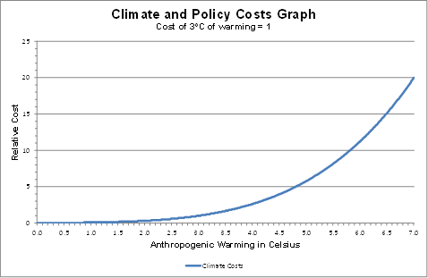
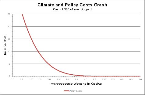
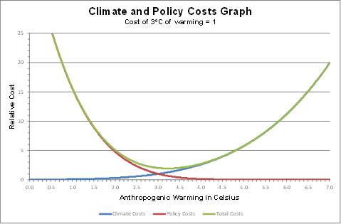
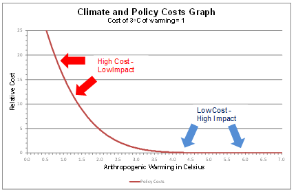
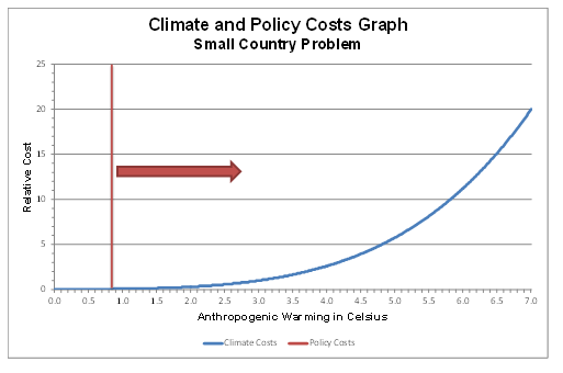
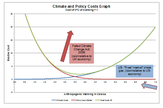
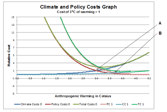
To his credit, Greg Craven in introducing both that human-caused climate change can have a trivial impact recognize that mitigating climate (taking action) is costly. But for the purposes of his decision grid he side-steps these issues to have binary positions on both. The decision is thus based on the belief that the likely consequences (costs) of catastrophic anthropogenic global warming then the likely consequences (costs) of taking action. A more sophisticated statement of this was from a report commissioned in the UK to justify the draconian climate action of the type Greg Craven is advocating. Sir Nicholas (now Lord) Stern’s report of 2006 (In the Executive Summary) had the two concepts of the warming and policy costs separated when it claimed

Using the results from formal economic models, the Review estimates that if we don’t act, the overall costs and risks of climate change will be equivalent to losing at least 5% of global GDP each year, now and forever. If a wider range of risks and impacts is taken into account, the estimates of damage could rise to 20% of GDP or more. In contrast, the costs of action – reducing greenhouse gas emissions to avoid the worst impacts of climate change – can be limited to around 1% of global GDP each year.

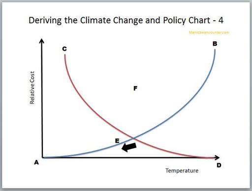
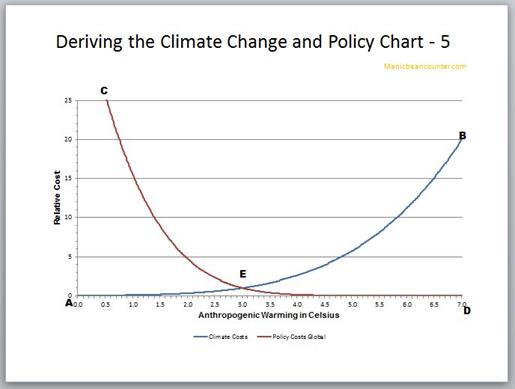
Craven has merely simplified the issue and made it more binary. But Stern has the same binary choice. It is a choice between taking costly action, or suffering the much greater possible consequences.  I will look at the policy issue first.

Action on Climate Change

The alleged cause of catastrophic anthropogenic global warming is (CAGW) is human greenhouse gas emissions. It is not just some people’s emissions that must be reduced, but the aggregate emissions of all 7.6 billion people on the planet. Action on climate change (i.e. reducing GHG emissions to near zero) must therefore include all of the countries in which those people live. The UNFCCC, in the run-up to COP21 Paris 2015, invited countries to submit Intended Nationally Determined Contributions (INDCs). Most did so before COP21, and as at June 2018, 165 INDCs have been submitted, representing 192 countries and 96.4% of global emissions. The UNFCCC has made them available to read. So these intentions will be sufficient “action” to remove the risk of CAGW? Prior to COP21, the UNFCCC produced a Synthesis report on the aggregate effect of INDCs. (The link no longer works, but the main document is here.) They produced a graphic that I have shown on multiple occasions of the gap between policy intentions on the desired policy goals. A more recent graphic is from the UNEP Emissions Gap Report 2017, published last October and

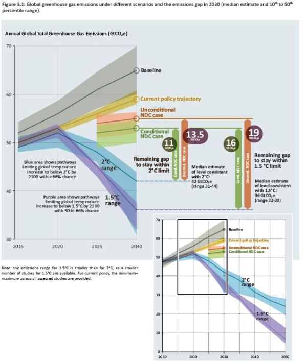
Figure 3 : Emissions GAP estimates from the UNEP Emissions GAP Report 2017

In either policy scenario, emissions are likely to be slightly higher in 2030 than now and increasing, whilst the policy objective is for emissions to be substantially lower than today and and decreasing rapidly. Even with policy proposals fully implemented global emissions will be at least 25% more, and possibly greater than 50%, above the desired policy objectives. Thus, even if proposed policies achieve their objective, in Greg Craven’s terms we are left with pretty much all the possible risks of CAGW, whilst incurring some costs. But the “we” is for 7.6 billion people in nearly 200 countries. But the real costs are being incurred by very few countries. For the United Kingdom, with the Climate Change Act 2018 is placing huge costs on the British people, but future generations of Britain’s will achieve very little or zero benefits.

Most people in the world live in poorer countries that will do nothing significant to constrain emissions growth if it that conflicts with economic growth or other more immediate policy objectives. In terms of the some of the most populous developing countries, it is quite clear that achieving the policy objectives will leave emissions considerably higher than today. For instance, China‘s main aims of peaking CO2 emissions around 2030 and lowering carbon emissions per unit of GDP in 2030 by 60-65% compared to 2005 by 2020 could be achieved with emissions in 2030 20-50% higher than in 2017. India has a lesser but similar target of reducing emissions per unit of GDP in 2030 by 30-35% compared to 2005 by 2020. If the ambitious economic growth targets are achieve, emissions could double in 15 years, and still be increasing past the middle of the century. Emissions in Bangladesh and Pakistan could both more than double by 2030, and continue increasing for decades after.

Within these four countries are over 40% of the global population. Many other countries are also likely to have emissions increasing for decades to come, particularly in Asia and Africa. Yet without them changing course global emissions will not fall.

There is another group of countries that are have vested interests in obstructing emission reduction policies. That is those who are major suppliers of fossil fuels. In a letter to Nature in 2015, McGlade and Ekins (The geographical distribution of fossil fuels unused when limiting global warming to 2°C) estimate that the proven global reserves of oil, gas and coal would produce about 2900 GtCO2e. They further estimate that the “non-reserve resources” of fossil fuels represent a further 8000 GtCO2e of emissions. The estimated that to constrain warming to 2C, 75% of proven reserves, and any future proven reserves would need to be left in the ground. Using figures from the BP Statistical Review of World Energy 2016 I produced a rough split by major country.

Figure 4 : Fossil fuel Reserves by country, expressed in terms of potential CO2 Emissions

Activists point to the reserves in the rich countries having to be left in the ground. But in the USA, Australia, Canada and Germany production of fossil fuels is not a major part of the economy. Ceasing production would be harmful but not devastating. One major comparison is between the USA and Russia. Gas and crude oil production are similar volumes in both countries. But, the nominal GDP of the US is more than ten times that of Russia. The production of both countries in 2016 was about 550 million tonnes or 3900 million barrels. At $70 a barrel that is around $275bn, equivalent to 1.3% of America’s GDP and 16% of Russia’s. In gas, prices vary, being very low in the highly competitive USA, and highly variable for Russian supply, with major supplier Gazprom acting as a discriminating monopolist. But America’s revenue is likely to be less than 1% of GDP and Russia’s equivalent to 10-15%. There is even greater dependency in the countries of the Middle East. In terms of achieve emissions targets, what is trying to be achieved is the elimination of the major source of the countries economic prosperity in a generation, with year-on-year contractions in fossil fuel sales volumes.

I propose that there are two distinct groups of countries that appear to have a lot lose from a global contraction in GHG emissions to near zero. There are the developing countries who would have to reduce long-term economic growth and the major fossil fuel-dependent countries, who would lose the very foundation of their economic output in a generation. From the evidence of the INDC submissions, there is now no possibility of these countries being convinced to embrace major economic self-harm in the time scales required. The emissions targets are not going to be met. The emissions gap will not be closed to any appreciable degree.

This leaves Greg Craven’s binary decision option of taking action, or not, as irrelevant. As taking action by a country will not eliminate the risk of CAGW, pursuing aggressive climate mitigation policies will impose net harms wherever they implemented. Further, it is not the climate activists who are making the decisions, but policy-makers countries themselves. If the activists believe that others should follow another path, it is them that must make the case. To win over the policy-makers they should have sought to understand their perspectives of those countries, then persuade them to accept their more enlightened outlook. The INDCs show that the climate activists gave failed in this mission. Until such time, when activists talk about the what “we” are doing to change the climate, or what “we” ought to be doing, they are not speaking about

But the activists have won over the United Nations, those who work for many Governments and they dominate academia. For most countries, this puts political leaders in a quandary. To maintain good diplomatic relations with other countries, and to appear as movers on a world stage they create the appearance of taking significant action on climate change for the outside world. On the other hand they are serving their countries through minimizing the real harms that imposing the policies would create. Any “realities” of climate change have become largely irrelevant to climate mitigation policies.

The Risks of Climate Apocalypse

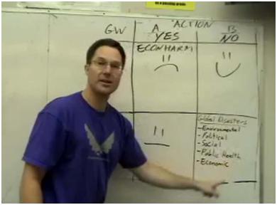
Greg Craven recognized a major issue with his original video. In the shouting match over global warming who should you believe? In How it all Ends (which was followed up by further videos and a book) Craven believes he has the answer.

Figure 5 : Greg Craven’s “How it all Ends”

It was pointed out that the logic behind the grid is bogus. As in Devil’s advocate guise Craven says at 3:50

Wouldn’t that grid argue for action against any possible threat, no matter how costly the action or how ridiculous the threat? Even giant mutant space hamsters? It is better to go broke building a load of rodent traps than risk the possibility of being hamster chow. So this grid is useless.

His answer is to get a sense of how likely the possibility of global warming being TRUE or FALSE is. Given that science is always uncertain, and there are divided opinions.

The trick is not to look at what individual scientists are saying, but instead to look at what the professional organisations are saying. The more prestigious they are, the more weight you can give their statements, because they have got huge reputations to uphold and they don’t want to say something that later makes them look foolish. 

Craven points to the “two most respected in the world“. The National Academy of Sciences (NAS) and the American Association for the Advancement of Science (AAAS). Back in 2007 they had “both issued big statements calling for action, now, on global warming“.  The crucial question from scientists (that is people will a demonstrable expert understanding of the natural world) is not for political advocacy, but whether their statements say their is a risk of climate apocalypse. These two bodies still have statements on climate change.

National Academy of Sciences (NAS) says

There are well-understood physical mechanisms by which changes in the amounts of greenhouse gases cause climate changes. The US National Academy of Sciences and The Royal Society produced a booklet, Climate Change: Evidence and Causes (download here), intended to be a brief, readable reference document for decision makers, policy makers, educators, and other individuals seeking authoritative information on the some of the questions that continue to be asked. The booklet discusses the evidence that the concentrations of greenhouse gases in the atmosphere have increased and are still increasing rapidly, that climate change is occurring, and that most of the recent change is almost certainly due to emissions of greenhouse gases caused by human activities.

Further climate change is inevitable; if emissions of greenhouse gases continue unabated, future changes will substantially exceed those that have occurred so far. There remains a range of estimates of the magnitude and regional expression of future change, but increases in the extremes of climate that can adversely affect natural ecosystems and human activities and infrastructure are expected.

Note, this is conjunction with the Royal Society, which is arguably is (or was) the most prestigious  scientific organisation of them all. It is what not said that is as important as what is actually said. They are saying that there is a an expectation that extremes of climate could get worse. There is nothing that solely backs up the climate apocalypse, but a range of possibilities, including changes somewhat trivial on a global scale. The statement endorses a spectrum of possible positions that undermines the binary TRUE /FALSE position on decision-making.

The RS/NAS booklet has no estimates of the scale of possible climate catastrophism to be avoided. Point 19 is the closest.

Are disaster scenarios about tipping points like ‘turning off the Gulf Stream’ and release of methane from the Arctic a cause for concern?

The summary answer is

Such high-risk changes are considered unlikely in this century, but are by definition hard to predict. Scientists are therefore continuing to study the possibility of such tipping points beyond which we risk large and abrupt changes.

This appears not to support Stern’s contention that unmitigated climate change will costs at least 5% of global GDP by 2100. Another context of the back-tracking on potential catastrophism is to to compare with  Lenton et al 2008 – Tipping elements in the Earth’s climate system. Below is a map showing the the various elements considered.

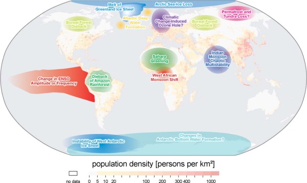
Figure 6 : Fig 1 of Lenton et al 2008, with explanatory note.

Of the 14 possible tipping elements discussed, only one makes it into the booklet six years later. Surely if the other 13 were still credible more would have been included in booklet, and less on documenting trivial historical changes.

American Association for the Advancement of Science (AAAS) has a video

Figure 7 : AAAS “What We Know – Consensus Sense” video


It starts with the 97% Consensus claims. After asking the listener on how many,  Marshall Sheppard, Prof of Geography at Univ of Georgia states.

The reality is that 97% of scientists are pretty darn certain that humans are contributing to the climate change that we are seeing right now and we better do something about it to soon.

There are two key papers that claimed a 97% consensus. Doran and Zimmerman 2009 asked two questions,

1. When compared with pre-1800s levels, do you think that mean global temperatures have generally risen, fallen, or remained relatively constant?

2. Do you think human activity is a significant contributing factor in changing mean global temperatures?

The second of these two responses was answered in the affirmative by 77 of 79 climate scientists. This was reduced from 3146 responses received. Read the original to find out why it was reduced.

Dave Burton has links to a number of sources on these studies. A relevant quote on Doran and Zimmerman is from the late Bob Carter

Both the questions that you report from Doran’s study are (scientifically) meaningless because they ask what people “think”. Science is not about opinion but about factual or experimental testing of hypotheses – in this case the hypothesis that dangerous global warming is caused by human carbon dioxide emissions.

The abstract to Cook et al. 2013 begins

We analyze the evolution of the scientific consensus on anthropogenic global warming (AGW) in the peer-reviewed scientific literature, examining 11 944 climate abstracts from 1991–2011 matching the topics ‘global climate change’ or ‘global warming’. We find that 66.4% of abstracts expressed no position on AGW, 32.6% endorsed AGW, 0.7% rejected AGW and 0.3% were uncertain about the cause of global warming. Among abstracts expressing a position on AGW, 97.1% endorsed the consensus position that humans are causing global warming. 

Expressing a position does not mean a belief. It could be an assumption. The papers were not necessarily by scientists, but merely authors of academic papers that involved the topics ‘global climate change’ or ‘global warming’. Jose Duarte listed some of the papers that were included in the survey, along with looking at some that were left out.

Neither paper asked a question concerning belief in future climate catastrophism. Sheppard does not make clear the scale of climate change trends from the norm, so the human-caused element could be insignificant. The 97% consensus does not include the policy claims.

The booklet is also misleading as well in the scale of changes. For instance on sea-level rise it states.

Over the past two decades, sea levels have risen almost twice as fast as the average during the twentieth century.

You will get that if you compare the tide gauge data with the two decades of satellite data. The question is whether those two sets of data are accurate. As individual tide gauges do not tend to show acceleration, and others cannot find statistically significant acceleration, the claim seems not to be supported.

At around 4.15 in the consensus video AAAS CEO Alan I. Leshner says

America’s leaders should stop debating the reality of climate change and start deciding the best solutions. Our What we Know report makes clear that climate change threatens us at every level. We can reduce the risk of global warming to protect out people, businesses and communities from harm. At every level from our personal and community health, our economy and our future as a global leader.  Understanding and managing climate change risks is an urgent problem. 

The statement is about combating the potential risks from CAGW. The global part of global warming is significant for policy. The United States share of global emissions is around 13% of global emissions. That share has been falling as America’s emissions have been falling why the global aggregate emissions have been rising. The INDC submission for the United States aimed as getting US emissions in 2025 at 26-28% of 2005 levels, with a large part of that reduction already “achieved” when the report was published. The actual policy difference is likely to be less than 1% of global emissions. So any reduction in risks with respect to climate change seems to be tenuous. A consensus of the best scientific minds should have been able to work this out for themselves.

The NAAS does not give a collective expert opinion on climate catastrophism. This is shown by the inability to distinguish between banal opinions and empirical evidence for a big problem. This is carried over into policy advocacy, where they fail to distinguish between the United States and the world as a whole.

Conclusions

Greg Laden’s decision-making grid is inapplicable to real world decision-making. The decision whether to take action or not is not a unitary one, but needs to be taken at country level. Different countries will have different perspectives on the importance of taking action on climate change relative to other issues. In the real world, the proposals for action are available. In aggregate they will not “solve” the potential risk of climate apocalypse. Whatever the actual scale of CAGW, countries who pursue expensive climate mitigation policies are likely to make their own people worse off than if they did nothing at all.

Laden’s grid assumes that the costs of the climate apocalypse are potentially far greater than the costs of action, no matter how huge. He tries to cut through the arguments by getting the opinions from the leading scientific societies. To put it mildly, they do not currently provide strong scientific evidence for a potentially catastrophic problem. The NAS / Royal Society suggest a range of possible climate change outcomes, with only vague evidence for potentially catastrophic scenarios. It does not seem to back the huge potential costs of unmitigated climate change in the Stern Review. The NAAAS seems to provide vague banal opinions to support political advocacy rather than rigorous analysis based on empirical evidence that one would expect from the scientific community.

It would appear that the binary thinking on both the “science” and on “policy” leads to a dead end, and is leading to net harmful public policy.

What are the alternatives to binary thinking on climate change?

My purpose in looking at Greg Laden’s decision grid is not to destroy an alternative perspective, but to understand where the flaws are for better alternatives. As a former, slightly manic, beancounter, I would (like the Stern Review  and William Nordhaus) look at translating potential CAGW into costs. But then weight it according to a discount rate, and the strength of the evidence. In terms of policy I would similarly look at the likely expected costs of the implemented policies, against the actual expected harms foregone. As I have tried to lay out above, the costs of policy and indeed the potential costs of climate change are largely subjective. Further, those implementing policies might be boxed in by other priorities and various interest groups jostling for position.

But what of the expert scientist who can see the impending on-coming catastrophes to which I am blind and to which climate mitigation will be useless? It is to endeavor to pin down the where, when, type and magnitude of potential changes to climate. With this information ordinary people can adjust their plans. The challenge for those who believe there are real problems is to focus on the data from the natural world and away from inbuilt biases of the climate community. But the most difficult part is from such methods they may lose their beliefs, status and friends.

First is to obtain some perspective. In terms of the science, it is worth looking at the broad range of  different perspectives on the Philosophy of Science. The Stanford Encyclopedia of Philosophy article on the subject is long, but very up to date. In the conclusions, the references to Paul Hoyningen-Huene’s views on what sets science apart seems to be a way out of consensus studies.

Second, is to develop strategies to move away from partisan positions with simple principles, or contrasts, that other areas use. In Fundamentals that Climate Science Ignores I list some of these.

Third, in terms of policy, it is worthwhile having a theoretical framework in which to analyze the problems. After looking at Greg Craven’s video’s in 2010, I developed a graphical analysis that will be familiar to people who have studied Marshallian Supply and Demand curves of Hicksian IS-LM. It is very rough at the edges, but armed with it you will not fall in the trap of thinking like the AAAS that US policy will stop US-based climate change.

Fourth, is to look from other perspectives. Appreciate that other people might have other perspectives that you can learn from. Or alternatively they may have entrenched positions which, although you might disagree with, are powerless to overturn. It should then be possible to orientate yourself, whether as an individual or as part of a group, towards aims that are achievable.

Kevin Marshall

1 Replicating Stern – The Costs of Climate Change and Policy Graph

One aspect of neoclassical economics that is extremely useful is the representation of an economic theory in a graphical form. Where would any introductory course be without Alfred Marshall’s supply and demand curves? For many years, the ideas of John Maynard Keynes’s ideas were synthesised in the Sir John Hicks’s IS-LM curves. These graphs have the advantage of enabling analysis of the logical consequences of changes in the overall context of the problem under consideration. In climate, there is a lot of shouting between the different camps, but what appears to be a complete inability to put the consequences of global warming and the mitigation policy option of globally constraining the growth of greenhouse gas emissions into their proper context. Therefore, when assumptions are changed, or new information becomes available, it is difficult to put those into the overall context of the “climate change” issue.

Sir Nicholas (now Lord) Stern’s report of 2006 (In the Summary of Conclusions) had the two ideas separated when it claimed

Using the results from formal economic models, the Review estimates that if we don’t act, the overall costs and risks of climate change will be equivalent to losing at least 5% of global GDP each year, now and forever. If a wider range of risks and impacts is taken into account, the estimates of damage could rise to 20% of GDP or more. In contrast, the costs of action – reducing greenhouse gas emissions to avoid the worst impacts of climate change – can be limited to around 1% of global GDP each year.


This leads to two offsetting sets of costs. The first is the “do-nothing approach” of letting greenhouse gas emissions spiral out of control, raising global temperatures by a number of degrees and throwing the weather systems out of control. The other is the policy costs of constraining the rise in emissions by switching to “cleaner” forms of living in general and energy-production in particular. It is should not be confused with a cost-benefit approach. Stern is proposing to exchange a very high set of costs in the distant future, with a much lower set of policy costs now. His proposal is not to incur costs in exchange for a stream of benefits (like when constructing a new motorway), but to minimize total costs of climate change and policy.

Constructing the graph

We are told by the climate scientists that some of the minor consequences of around 0.8oC of warming over the last century are already visible. But their climate models project this is utterly insignificant compared to what will happen if greenhouse gases continue to increase unchecked for the next century or more. The large increases in temperature – around 4oC to 7oC or higher – would cause massive disruption to the climate system. It is fair to say that as global temperatures increase, these costs would increase exponentially. These “costs” are in the broadest sense. They are not just the human costs of property damage, failed harvests, population migrations and land being submerged by rising seas. These include the damage to the eco-systems and species extinction. Assuming a top end of 7oC the cost curve would look something like this.

The relative cost scales 7oC of warming are set to be twenty times the costs of constraining global warming to 3oC, or the mid-range of estimates by the IPCC for a doubling of CO2 from pre-industrial levels of 280ppm, and an approximate policy target.

Conversely, the cost of stopping any more warming will be huge. Hugely aggressive policies would quickly stop any increases in emissions and could bring about major reductions. But such policies would bring to a halt the fast-growing economies of China and India, and would considerably worsen the recession in much of Europe. However, it is possible to postulate that low-cost policies that give the odd nudge here and there over a long period could reap large rewards. In line with climate costs, I have set the relative cost of constraining the rise in global temperatures to 3oC above the pre-industrial levels to 1. So the curve might look like the one below.

Combining the two curves gives a total cost graph.

The total costs curve is derived by the addition of the climate and policy cost curves.

This replicates Stern’s statement above. The “do-nothing” scenario is ten times more expensive than the optimal cost-minimization scenario.

Some points to note.

First is that the total cost curve has quite a wide minimum area. Even if a lot of the main policy targets are missed, doing something looks to be far better than doing nothing at all.

Second, is that cost minimization strategy is at a higher temperature level than the intersection of the curves. However, a risk-averse strategy (which most people would expect in avoiding a prospective global catastrophe) would aim for a somewhat lower temperature increase.

Third is that “policy” should be called mitigation policy. That is preventing climate change costs from occurring by constraining the rise in greenhouse gases. As will be seen later, the alternative (or complementary) adaptation policies are included within the climate costs curve. The full reasons will be explained later, but the main one is that climate mitigation is something that, by definition, needs to be tackled at a global level, whereas adaptation can be done at the local, country or regional levels.

Fourth, is a clear separation of mitigation policy considerations from the projections of climate science. Yet new information from the science and policy areas can be put into a total context of acting in the best interests of the planet and the human population.

Fifth, an issue with the policy curve is the change in gradient. There must exist a set of policy options which are low cost, high impact (LC-HI) as well as the high cost, low impact (HC-LI). There are two possible types of policies which should be avoided. First are those with costs, but with zero impact (C-ZI) and second are those with a net negative impact (NNI).

Sixth, any look at climate projections and policy options show they are all over the place. The assumptions of single curves are highly restrictive ones. But like in

Finally, on climate costs there is an issue with projections about future costs. The data we have is from less than one degree of warming, and a minute fraction of projected costs. As shall be shown, the handling of this issue is crucial.

Kevin Marshall

2 Climate Change Policy Choices

The risks from policy are becoming increasingly well-known. The question is how to manage these risks. Assuming there is a genuine problem, which is possible to overcome through policy, what are we doing to make a real difference? The policy curve gradient assumes there must exist a set of policy options which are low cost, high impact (LC-HI) as well as the high cost, low impact (HC-LI).

There are two possible types of policies which should be avoided. First are those with costs, but with zero impact (C-ZI) and second are those with a net negative impact (NNI). All of these costs may include unintended consequences, which may not be fully recognized.

The choice is quite clear. Policy creation and policy implementation requires a high degree of focus in driving through effective emission reductions.


3 The Mitigation Policy Curve – Part 1

One of the aspects of neoclassical economics is that you make a whole host of assumptions, some of which are highly unrealistic. This enables one to look at the consequences of removing or changing the assumptions one at a time. For this exercise, let us assume the global cost curves are correct. That is to assume that if no policy is enacted that there will be significant global warming with catastrophic consequences for the planet and the people upon it, whilst there are a set of feasible global policies that mitigate against this.

As stated above, for a viable mitigation policy curve to exist, there must exist a set of low cost, high impact (LC-HI) policies. If you believe, as I do, that public policy should aim to make the maximum positive difference, and at a minimum to avoid net harm, then for climate change there is a duty of care in creation and implementation of policy that this truly happens.

The Small Country Problem

A small country is faced with the same climate cost curve as the entire planet. That is, if nothing is done to constrain the growth in greenhouse gas (GHG) emissions this country will face the same escalating costs of climate change. The only difference is that this cost is no longer relative to total gross world product (GWP), but relative to its own GDP. Assuming that the country’s emissions are an insignificant part of the total world amount to begin with, no matter how effective that country is in constraining its own emissions growth path, or even in cutting its total emissions, its policy cost curve will be vertical. It will move to the right with the relentless rise in global temperatures.

The total costs curve, for any temperature level will simply be the addition of the climate change costs and the money spent on emissions reductions.

The more spent by this small country, the greater its prestige in the green movement for unilaterally leading the way on “saving the planet.” But if nobody follows the small country’s example, then its “conspicuous impoverishment”(1) will be in vain.

Avoiding the small country example

How do we avoid the small country example, where the total costs are just added to by wasted effort on cutting emissions?

The standard answer is along the lines of saying if everybody does their bit, with the rich countries taking the lion’s share of the responsibility, then everything will be just fine. What is more, Britain already has some of most draconian emissions reductions targets in the world, as imposed by the Climate Change Act 2008 and others, such as the EU and Australia are also contributing. The small country argument does not hold.

The minority of countries pursuing emission reduction policies I will term the PC1 group. Still assume for the moment that the policy cost curve is correct. The current issue is to enlarge that group to make it the PC2 group. Eventually it is to convince every country to join making the policy curve truly global. As the group enlarges the policy curve shifts to the left.

If all PC1 countries commit to restrain global warming to 3oC, then they can only do so by crippling their economies. The relative cost is a global one after all. They still could cripple their economies if they went to the climate costs equal policy costs point. If the PC1 countries accounted for 25% of GWP, then they would have a benefit a quarter of all the countries acting together. So should the in the economic interests of an outsider country to help create an enlarged group PC2, that represents 50% of GWP? The PC1 group will rid the planet of over 75% of the climate change costs. The PC2 group could halve that again.

Would it be in the economic interests of a country to join the PC2 group, or stay outside?

My Excel graph gets a bit blocky here – sorry.

Let’s do the maths, with approximate numbers. Enlarging the policy-enacting group moves from point A to point B.

PC1 group members have a climate cost of 3.1 plus a policy cost of 3.1/25% = 12.4

Non PC1 members have a climate cost of 3.1 = 3.1

PC2 group members have a climate cost of 1.7 plus a policy cost of 1.7/50% = 5.1

Non PC1 members have a climate cost of 1.7 = 1.7.

So to join the enlarged PC2 group, would increase costs from 3.1 to 5.1. To stay outside the policy countries would be better for the citizens of that country, even if there is a workable policy to adopt and the clear prospect of catastrophic global warming if no mitigation policy is enacted.

Later arguments on the effectiveness of policy and prospective costs of climate will make this choice look even more unambiguous. This aspect of all countries not acting together to share proportionately the costs has not, as far as I am aware, been seriously looked at in the literature. This is why the annual COP meetings – conferences in exotic locations – will never get anywhere. Any leaders that are persuaded to join the policy-enactors, unless their country will be disproportionately made worse by climate change, are acting against their own national interests.


Policy Risk

Policies carry risks. There is a risk of them not being effective, and costs running out of control. There is also a risk of a ratchet effective. That is once the policy is implemented, vested interests are created that make it very difficult to withdraw the policy even if results fall far short of those expected. The above assumes policy success. Policy failure within PC1 countries will demonstrate to potential PC2 countries that they should avoid adopting mitigation policies, no matter how great they believe in the looming climate catastrophe.


  1. Thorstein Veblen attacked in the rich for the “conspicuous consumption”. The “conspicuous impoverishment” of the global warming movement is a variant on this, the difference is that the “prestige” that Veblen went to those wasting their money. The “prestige” heaped on the unilateralist country by the green movement on those implementing the policy and not those suffering the policy consequences.


4 The Mitigation Policy Curve – Part 2 – Counter-Examples

In the first part on the mitigation policy curve I looked at

  • The Small Country Problem. How one small country acting unilaterally will make an insignificant impacts of global climate change.
  • How it is very likely to be against the economic interests of any country to join the small group of countries already with climate mitigation policies.

In this section I will look at two examples that go completely against logical thinking. There can be instances (like in Britain) where bold policies increase global warming at great cost to that economy, but the shale gas, which constrains global warming at net benefit to the gas-producing country?

To see the effect of policy, there is a need for analysis both at the front-end (prior to implementation), during and after. The question is about the gradient of the policy cost curve, at the point

Policy increasing global emissions?

We know that policy countries are in a minority of countries. With the structure of global growth this amount will fall.

Look at the long-term. Implementing a policy, you are saying to businesses that, ceteris paribus, your energy costs are going to rise year-on-year relative to those in non-policy countries. There will be a bigger incentive to make technological efficiency gains in these countries, but those gains can be transplanted to non-policy countries. In this global emissions may decrease more rapidly than they would have done, but the policy countries bear well over 100% of the costs and it becomes a policy benefit to the non-policy countries. By implication they will achieve around 200% of the global decline in emissions.

Question is, will it be more or less than 200% of the decline? Could it be that the policy countries energy-efficient factories are replaced by less energy-efficient factories in the non-policy countries?
There is some economic theory needed here. The Solow growth model shows a technological growth curve. Developing countries can achieve rapid growth by adapting to higher-productivity by adapting existing technologies. Their lower-unit labour costs will enable to undercut the more advanced economies, but the growth in these economies will grow the global economy as well. Most of this is unit labour costs. But by adapting previous generation technologies and exploiting labour costs less than a tenth those of the rich countries, they can under-cut the rich world. Greater technological advance is mostly in unit labour costs, but it can also mean lower unit energy costs. The portion of global output transferred from the rich countries to the poorer developing countries could result in higher total energy use, and ceteris paribus, higher CO2 emissions.

What is clear is that policy countries will increase unit energy costs. There is a two-pronged approach in Britain. The European-wide carbon-trading scheme will restrict supply of energy, bidding up the price. But also renewables cost more than fossil fuels. So the two-pronged approach doubly increases unit energy costs. Increasing unit energy costs accelerates the switching of manufacturing to developing countries, mostly China. The blue bit above postulates that energy per unit of output is globally could increase. But that is part of the problem. China has much higher CO2 emissions per unit of output as Britain. If Britain’s aggressive rush to renewables is successful, then this gap will increase, as much of Chinese energy output is from coal. A de-carbonised British economy will also be a de-industrialised one. But overall global emissions will have increased through switching of output to China.

The biggest cost of the policy for Britain is nothing to do with switching low-CO2 emitting production to high CO2 emitting countries. It is the restriction on economic growth. Loss of jobs from manufacturing, and pushing up higher energy costs elsewhere constrains growth. Due to the long-term consequences of that pushes policy costs through the roof. In the sectors where jobs are lost overseas, the policy curve is positive. If British Climate Change Act 2008 is massively unsuccessful in meeting the carbon targets, it could be a very expensive policy to increase global CO2 emissions.

The Shale-Gas Counter Example

In the USA, a consequence of the shale gas revolution has been to drastically reduce unit energy costs to industry. But also there has been a switch away from coal. As CO2 emissions of gas are around half that of coal, US CO2 emissions have been falling with electricity prices. The US is enjoying both cheaper and cleaner energy. Consequently, some chemical factories that relocated to China have returned to the USA. China has a greater proportion in its electricity production than USA, and the gap is widening. So the switching of a factory from USA reduces global CO2 emissions, even though the total energy usage remains the same.

Let me show this graphically.

Suppose (as is likely at present), the Climate Change Act 2008 falls a long way short of its target but unintentionally moves a substantial part of manufacturing to China through higher costs. For Britain this will be a large cost relative to British, but may be a net contributor to global warming. The policy curve points gets a positive slope! Conversely, “free market” shale gas in the USA has constrained global carbon emissions doubly by reducing US carbon emissions per unit of output, and switching production from China, where carbon emissions per unit of output are higher. It is having positive benefits on the US economy as well (hence negative costs), whilst constraining (slightly) the top-end of global warming.

5 The Climate Cost Curve

This is a draft proposal in which to frame our thinking about the climatic impacts of global warming, without getting lost in trivial details, or questioning motives. It is an updated version of a draft posted on 26/10/2012.

The continual rise in greenhouse gases due to human emissions is predicted to cause a substantial rise in average global temperatures. This in turn is predicted to lead severe disruption of the global climate. Scientists project that the costs (both to humankind and other life forms) will be nothing short of globally catastrophic.

That is

CGW= f {K}                 (1)

The costs of global warming, CGW are a function of the change in the global average surface temperatures K. This is not a linear function, but of increasing costs per unit of temperature rise. That is

CGW= f {Kx} where x>1            (2)

Graphically

The curve is largely unknown, with large variations in the estimate of the slope. Furthermore, the function may be discontinuous as, there may be tipping points, beyond which the costly impacts of warming become magnified many times. Being unknown, the cost curve is an expectation derived from computer models. The equation thus becomes

E(CGW)= f {Kx}                (3)

The cost curve can be considered as having a number of interrelated elements of magnitude M, time t and likelihood L. There are also the adaptation costs/benefits (which should lead to a planned credit) along with the costs involved in taking actions based on false expectations. Over a time period, costs are normally discounted by r. Then there are two subjective factors – The collective risk factor R, and, when considering a policy response, a weighting W should be given to the scientific evidence. That is

E(CGW)=f {M,1/t,L,A,│Pr-E()│,r,R,W}    (4)

Magnitude M is the both severity and extent of the impacts on humankind or the planet in general in a physical sense.

Time t is highly relevant to the severity of the problem. Rapid changes in conditions are far more costly than gradual changes. Also impacts in the near future are more costly than those in the more distant future due to the shorter time horizon to put in place measures to lessen those costs.

Likelihood L is also relevant to the issue. Discounting a possible cost that is not certain to happen by the expected likelihood of that occurrence enables due unlikely but catastrophic events to be considered alongside near certain events.

Adaptation A is for a project to adapt to the changed climate, to lessen or null the costs. It is the difference between the actual costs spent and the climate impacts saved. Upon completion, a project should have a net credit value.

│Pr-E()│ is the difference between the predicted outcome, based on the best analysis of current data at the local level, and the expected outcome, that forms the basis of adaptive responses. It can create a cost in two ways. If there is a failure to predict and adapt to changing conditions then there is a cost. If there is adaptation to an anticipated future condition that does not emerge, or is less severe than forecast, there is also a cost. │Pr-E()│= 0 when the outturn is exactly as forecast in every case. Given the uncertainty of future outcomes, there will always be costs incurred if the climate cost savings from adaptation is a unitary value. If there are a range of possible scenarios, then this value could be a credit.

Discount rate r is a device that recognizes that people prioritize according to time horizons. Discounting future costs or revenue enables us to evaluate the discount future alongside the near future.

Collective risk factor R, is the risk preference weighting. If policy-makers assume a collective risk-neutral position, then this weighting will be 1. Risk lovers – the gamblers and many self-made billionaires – have a weighting of less than one. Those who take out insurance are risk averse. Insurance gives a certain premium to compensate if a much greater probabilistic loss occurs. For instance, the probability of a £200,000 house being completely destroyed in a year is around 1 in 10,000. So the expected loss is just £20 in any year. Most people are risk averse when it comes to their most valuable asset, so would pay a premium of far greater than £20 compensate for this unlikely loss. With respect to potential catastrophes, we usually expect governments to take a risk-averse approach. That is to potentially spend more on certain costs (like flood defences) than the total expected losses from letting catastrophes from happening. For any problem on a vast scale, we need to articulate the risk preference weighting. The “precautionary principle”, used in arguing for tough and immediate mitigation policies, effectively creates a collective risk factor many times greater than 1. NB, as the costs of climate change will increase with time, a risk averse weighting is the equivalent of a negative discount rate r. That is, you could assume R = f {-r}.

Finally the Weighting (W) is concerned with the strength of the evidence. How much credence do you give to projections about the future? Here is where value judgements come into play. I believe that we should not completely ignore alarming projections about the future for which there is highly circumstantial evidence, but neither should we accept such evidence as the only possible future scenario. In fact, by its very nature the “evidence” will be highly circumstantial. Consider the costs of climate change graph again. The data we have (which needs to converted into evidence) is for a very short section, and for miniscule fluctuations in costs, compared to the predicted catastrophe.

This leads to a vast area of evidence quality as

  • Small errors or biases in temperature measurement will have huge impacts on future projections. (Impacts on historical climate sensitivity)
  • Small errors or biases in distinguishing between natural and human-caused extreme weather events or short-run climatic changes will have huge impacts on projected costs.

If we assume that some sort of climate catastrophe is going to happen, convincing an independent third-party could include

  • Science building a clear track record of short-run predictive successes, both on warming trends and damage impacts.
  • Learning from the errors and exaggerations.
  • Be very clear as to the quality and relevance of the evidence.
  • Corroborating evidence. Show the coherence of one part of the picture with another. For instance, trying to reconcile with estimates of polar ice cap rate of melt with the rate of sea level rise reveals some very interesting questions.
  • Corroboration of between different techniques and evaluation methods.
  • For a junior science, show the underlying methodology draws upon the best of the mature sciences and philosophies of science.

The prediction of catastrophe is highly emotive. There are comparisons here with the justice system in has Britain failed where there are highly emotive crimes, for instance the IRA bringing their bombing campaign to the British mainland in the early 1970s.

  • Clear separation of the understandable emotion, from the evidence gathering.
  • Developing, and continually improving, quality standards for evidence gathering
  • A dim view taken for tampering with, or suppression of evidence.
  • A dim view taken on influencing the jury.
  • Allowing the accused a strong defence. The lack of any credible defence argument, despite a strong defence team, will remove any “reasonable doubt” in the minds of the jury, where the accused is in denial of the overwhelming evidence of their guilt.

6 A halving of climate sensitivity

Lord Lawson, in a spirited attack on the Energy Bill passing through parliament, said in the House of Lords on 18th June 2013

There is an emerging consensus among scientists that the climate sensitivity of carbon is probably less than they thought. That means, importantly, that any dangers from warming, if they occur, are postponed well into the next century. It means that there is no urgency to go ahead in this way, not only because the uncertainties are in the distant future but because we have no idea what technologies will develop over the next 100 years.

The analysis I have developed shows Lord Lawson understates how significant the climate sensitivity issue to the problem of catastrophic warming and mitigation policy.

In my analysis, the maximum warming would be 7oC. There can be a case for warming topping out at some level, as

  • There are diminishing returns to increases in greenhouse gas on temperature.
  • There are diminishing returns at some point for unit rises in emissions on levels of GHGs. That is, higher levels of GHGs in the atmosphere will lead to higher levels of absorption.

I will assume that climate sensitivity is halved, but will assume that temperatures eventually reach 5oC above pre-industrial levels.

The simple curve to work out the consequences is the policy curve. Any constraint of greenhouse gas levels will only have half the impact on temperature. The policy curve will shift to the right to PC1.

The climate costs curve is somewhat more difficult. The elements to consider in the curve are

E(CGW)=f {M,1/t,L,A,│Pr-E()│,r,R,W}

I have highlighted the elements to consider.

Time t will be doubled. Warming rates will therefore be halved. Some of the harmful consequences of warming are from unprecedented rapid change. For many animals and plants, it is speculated sudden change is much more damaging than a slower change. More importantly, sudden changes in average temperature could jolt climate systems into different patterns. Savannahs could become deserts, or the monsoon could shift. Another aspect to consider is that rapid warming of the tundra could release massive amounts of CH4 into the atmosphere, further accelerating warming. Or rapid warming could lead to rapid disintegration and breakup of the polar ice caps, leading to rapid acceleration of sea level rise. The slower warming will make us much less likely to cross these climate tipping points.

Adaptations A
can be phased in more gradually. For instance, with sea level rise, the Thames Barrier will no longer be adequate. A replacement to last 50 years will need to be much less extensive. If warming causes crop yields to fall by increased drought there is more time to adjust.

With changes happening more slowly, (and less chaotically), the adaptation cost errors, │Pr-E()│, are likely to be less.

For any positive rate of discount r, then the current net present value will be lower for the much extended warming period. However, as Stern had a discount value of not much different to zero, allowing for a discount rate would totally cover the other issues.

For all of these reasons, the climate cost curve will move down to CC1 and total cost curve to TC1. The point where policy costs equals climate change costs moves from A to B. That is at a significantly higher temperature, and for a much lower level of policy cost.

I have steered away from the weighting W issues. But given that sensitivity is a core issue that the climate models have got consistently wrong, then any weighting given to other predictions should be viewed with greater scepticism.

7 Appendix – Deriving the Policy and Forecast Graph

In the introduction, the derivation of the graph to replicate the claim that the costs of catastrophic global warming will be many times greater than mitigation policy costs was logically incomplete. This is a derivation of the two cost functions from a series of PowerPoint slides, which I find somewhat more satisfactory.

Slide 1

First draw two axis’s – for temperature and relative cost.

Slide 2

Next, add in five points.

A. If there had been no rise in human greenhouse gases, there would be no rise in temperatures and thus no consequential costly climate impacts.

B. With “business as usual”, there will be a huge amount of warming, with hugely costly consequential climate impacts.

C. Globally, policy could be used to stop any further rise in greenhouse gases, but with huge global cost.

D. No policy and no policy costs.

E. Intersection of two curves, which in Stern’s view is at the point of constraining warming to about 3 degrees above pre-twentieth century levels.

Slide 3

Connecting up the points AB (climate costs) and CD (Policy costs) with straight lines (linear functions), creates an intersection at point F.

To replicate Stern, we need cost functions that intersect at point E. That is the climate cost curve connects AEB and the policy costs curve connects CED.

Slide 4

Drawing curves within PowerPoint is beyond my current skills. Simple curves have symmetrical properties. The required cost curves do not have such properties.

Slide 5

Above is the actual graph used.

Slide 6

On my graphs the cost curves are unstable functions

For climate costs

RC = f(T4)

For policy costs

RC = f((10-T)5)

To justify policy

  1. Must have reliable consequences of warming beyond human experience. Climate models must be robust for the high temperature rise forecast and have a phenomenal degree of precision on the shorter-term cost impact forecasts.
  2. Must be sure that got achievable high-impact low-cost policies, with a highly results-driven approach to policy implementation.