Milk loss yields down to heat stress

Last week, Wattupwiththat post “Climate Study: British Children Won’t Know What Milk Tastes Like”. Whilst I greatly admire Anthony Watts, I think this title entirely misses the point.
It refers to an article at the Conservation “How climate change will affect dairy cows and milk production in the UK – new study” by two authors at Aberystwyth University, West Wales. This in turn is a write up of a Plos One article published in May “Spatially explicit estimation of heat stress-related impacts of climate change on the milk production of dairy cows in the United Kingdom“. The reason I disagree is that even with very restrictive assumptions, this paper shows that even with large changes in temperature, the unmitigated costs of climate change are very small. The authors actually give some financial figures. Referring to the 2190s the PLOS One abstract ends:-

In the absence of mitigation measures, estimated heat stress-related annual income loss for this region by the end of this century may reach £13.4M in average years and £33.8M in extreme years.

The introduction states

The value of UK milk production is around £4.6 billion per year, approximately 18% of gross agricultural economic output.

For the UK on average Annual Milk Loss (AML) due to heat stress is projected to rise from 40 kg/cow to over 170 kg/cow. Based on current yields it is from 0.5% to 1.8% in average years. The most extreme region is the south-east where average AML is projected to rise from 80 kg/cow to over 320 kg/cow. That is from 1% to 4.2% in average years. That is, if UK dairy farmers totally ignore the issue of heat stress for decades the industry could see average revenue losses from heat stress rise on average from £23m to £85m. The financial losses are based on constant prices of £0.30 per litre.

With modeled estimates over very long periods, it is worth checking the assumptions.

Price per liter of milk

The profits are based upon a constant price of £0.30 a liter. But prices can fluctuate according to market conditions. Data on annual average prices paid is available from AHDB Dairy, ” a levy-funded, not-for-profit organisation working on behalf of Britain’s dairy farmers.” Each month, since 2004, there are reported the annual average prices paid by dairies over a certain size available here. That is 35-55 in any one month. I have taken the minimum and maximum prices for reported in June each year and shown in Figure 1.

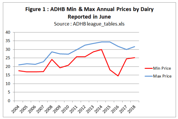
Even annual average milk prices fluctuate depending on market conditions. If milk production is reduced in summer months due to an unusual heat wave causing heat stress, ceteris paribus, prices will rise. It could be that a short-term reduction in supply would increase average farming profits if prices are not fixed. It is certainly not valid to assume fixed prices over many decades.

Dumb farmers

From the section in the paper “Milk loss estimation methods

It was assumed that temperature and relative humidity were the same for all systems, and that no mitigation practices were implemented. We also assumed that cattle were not significantly different from the current UK breed types, even though breeding for heat stress tolerance is one of the proposed measures to mitigate effects of climate change on dairy farms.

This paper is looking at over 70 years in the future. If heatwaves were increasing, so yields falling and cattle were suffering, is it valid to assume that farmers will ignore the problem? Would they not learn from areas with more extreme heatwaves in summer elsewhere such as in central Europe? After all in the last 70 years (since the late 1940s) breeding has increased milk yields phenomenally (from AHDB data, milk yields per cow have increased 15% from 2001/2 to 2016/7 alone) so a bit of breeding to cope with heatwaves should be a minor issue.

The Conversation article states the implausible assumptions in a concluding point.

These predictions assume that nothing is done to mitigate the problems of heat stress. But there are many parts of the world that are already much hotter than the UK where milk is produced, and much is known about what can be done to protect the welfare of the animals and minimise economic losses from heat stress. These range from simple adaptations, such as the providing shade, to installing fans and water misting systems.

Cattle breeding for increased heat tolerance is another potential, which could be beneficial for maintaining pasture-based systems. In addition, changing the location of farming operations is another practice used to address economic challenges worldwide.

What is not recognized here is that farmers in a competitive market have to adapt in the light of new information to stay in business. That is the authors are telling farmers what they will be fully aware of to the extent that their farms conform to the average. Effectively assuming people and dumb, then telling them obvious, is hardly going to get those people to take on board one’s viewpoints.

Certainty of global warming

The Conversation article states

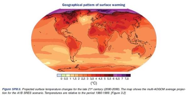
Using 11 different climate projection models, and 18 different milk production models, we estimated potential milk loss from UK dairy cows as climate conditions change during the 21st century. Given this information, our final climate projection analysis suggests that average ambient temperatures in the UK will increase by up to about 3.5℃ by the end of the century.

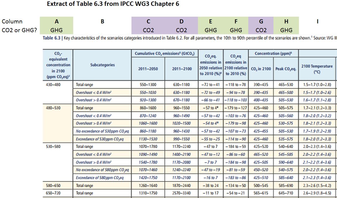
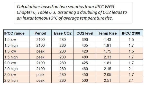
This warming is consistent with the IPCC global average warming projections using RCP8.5 non-mitigation policy scenario. There are two alternative, indeed opposite, perspectives that might lead rational decision-makers to think this quantity of warming is less than certain.

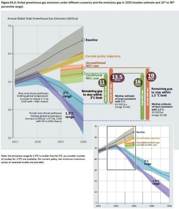
First, the mainstream media, where the message being put out is that the Paris Climate Agreement can constrain global warming to 2°C or 1.5°C above the levels of the mid-nineteenth century. With around 1°C of warming already if it is still possible to constrain additional global warming to 0.5°C, why should one assume that 3.5°C of warming for the UK is more than a remote possibility in planning?

Second, one could look at the track record of global warming projections from the climate models. The real global warming scare kicked-off with James Hansen’s testimony to Congress in 1988. Despite actual greenhouse gas emissions being closely aligned with rapid warming, actual global warming has been most closely aligned with the assumption of the impact of GHG emissions being eliminated by 2000. Now, if farming decision-makers want to still believe that emissions are the major driver of global warming, they can find plenty of excuses for the failure linked from here. But, rational decision-makers tend to look at the track record and thus take consistent decision-makers with more than a pinch of salt.

Planning horizons

The Conversation article concludes

(W)e estimate that by 2100, heat stress-related annual income losses of average size dairy farms in the most affected regions may vary between £2,000-£6,000 and £6,000-£14,000 (in today’s value), in average and extreme years respectively. Armed with these figures, farmers need to begin planning for a hotter UK using cheaper, longer-term options such as planting trees or installing shaded areas.

This compares to the current the UK average annual dairy farm business income of £80,000 according to the PLOS One article.

There are two sides to investment decision-making. There are potential benefits – in this case avoidance of profit loss – netted against the potential benefits. ADHB Dairy gives some figures for the average herd size in the UK. In 2017 it averaged 146 cows, almost double the 75 cows in 1996. In South East England, that is potentially £41-£96 a cow, if the average herd size there is same as the UK average. If the costs rose in a linear fashion, that would be around 50p to just over a pound a year per cow in the most extreme affected region. But the PLOS One article states that costs will rise exponentially. That means there will be no business justification for evening considering heat stress for the next few decades.

For that investment to be worthwhile, it would require the annual cost of mitigating heat stress to be less than these amounts. Most crucially, rational decision-makers apply some sort of NPV calculation to investments. This includes a discount rate. If most of the costs are to be incurred decades from now – beyond the working lives of the current generation of farmers – then there is no rational reason to take into account heat stress even if global warming is certain.

Summary

The Paper Spatially explicit estimation of heat stress-related impacts of climate change on the milk production of dairy cows in the United Kingdom makes a number of assumptions to reach its headline conclusion of decreased milk yields due to heat stress by the end of the century. The assumption of constant prices defies the economic reality that prices fluctuate with changing supply. The assumption of dumb farmers defies the reality of a competitive market, where they have to respond to new information to stay in business. The assumption of 3.5°C warming in the UK can be taken as unlikely from either the belief Paris Climate Agreement with constrain further warming to 1°C or less OR that the inability of past climate projections to conform to the pattern of warming should give more than reasonable doubt that current projections are credible.  Further the authors seem to be unaware of the planning horizons of normal businesses. Where there will be no significant costs for decades, applying any sort of discount rate to potential investments will mean instant dismissal of any consideration of heat stress issues at the end of the century by the current generation of farmers.

Taking all these assumptions together makes one realize that it is quite dangerous for specialists in another field to take the long range projections of climate models and apply to their own areas, without also considering the economic and business realities.

Kevin Marshall 

“Were going to miss the 2°C Warming target” study and IPCC AR5 WG3 Chapter 6

WUWT had a post on 22nd January

Study: we’re going to miss (and overshoot) the 2°C warming target

This comment (from a University of Southhampton pre-publication news release) needs some explanation to relate it to IPCC AR5.

Through their projections, Dr Goodwin and Professor Williams advise that cumulative carbon emissions needed to remain below 195-205 PgC (from the start of 2017) to deliver a likely chance of meeting the 1.5°C warming target while a 2°C warming target requires emissions to remain below 395-455 PgC.

The PgC is peta-grams of Carbon. For small weights, one normally uses grams. For larger weights one uses kilograms. For still larger weights one uses tonnes. Under the Imperial measurement system, one uses ounces, pounds and tons. So one peta-gram is a billion (or giga) tonne.
Following the IPCC’s convention, GHG emissions are expressed in units of CO2, not carbon. Other GHGs are expressed in CO2e. So 1 PgC = 3.664 GtCO2e.

So the emissions from the start of 2017 are 715-750 GtCO2e for 1.5°C of warming and 1447-1667 GtCO2e for 2°C of warming. To make comparable to IPCC AR5, (specifically to table 6.3 from IPCC AR5 WG3 Chapter 6 p431), one needs to adjust for two things – the IPCC’s projections are from 5 years earlier, and for CO2 emissions only, about 75% of GHG emissions.

The IPCC’s projections of CO2 emissions are 630-1180 GtCO2 for 1.5-1.7°C of warming and 960-1550 GtCO2e for 1.7-2.1°C of warming.

With GHG emissions roughly 50 GtCO2e a year and CO2 emissions 40 GtCO2 a year, from the IPCC’s figures updated from the start of 2017 and expressed in GtCO2e are 570-1300 GtCO2e for 1.5-1.7°C of warming and 1010-1800 GtCO2e for 1.7-2.1°C of warming.

Taking the mid-points of the IPCC’s and the Goodwin-Williams figures, the new projections are saying that at current emissions levels, 1.5°C will be breached four years earlier, and 2°C will be breached one year later. Only the mid-points are 1.6°C and 1.9°C, so it makes no real difference whatsoever. The Goodwin-Williams figures just narrow the ranges and use different units of measure.

But there is still a major problem. Consider this mega table 6.3 reproduced, at lower quality, below.

Notice Column A is for CO2 equivalent concentration in 2100 (ppm CO2eq). Current CO2 levels are around 405 ppm, but GHG gas levels are around 450 ppm CO2eq. Then notice columns G and H, with a joint heading of Concentration (ppm). Column G is for CO2 levels in 2100 and Column H is for CO2 equivalent levels. Note also that for the first few rows of data, Column H is greater than Column A, implying that sometime this century peak CO2 levels will be higher than at the end of the century, and (subject to the response period of the climate system to changes in greenhouse gas levels)  average global temperatures could (subject to the models being correct) exceed the projected 2100 levels. How much though?

Using a magic equation at the skeptical science blog, and (after correcting to make a doubling of CO2 convert to exactly 3°C of warming) assume that all changes in CO2 levels instantly translate into average temperature changes. Further, I assume that other greenhouse gases are irrelevant to the warming calculation, and peak CO2 concentrations are calculated from peak GHG, 2100 GHG, and 2100 CO2 concentrations. I derived the following table.

The 1.5°C warming scenario is actually 1.5-1.7°C warming in 2100, with a mid-point of 1.6°C. The peak implied temperatures are about 2°C.

The 2°C warming scenario is actually 1.7-2.1°C warming in 2100, with a mid-point of 1.9°C. The peak implied temperatures are about 2.3°C, with 2.0°C of warming in 2100 implying about 2.4°C peak temperature rise.

So when the IPCC talk about constraining temperature rise, it is about projected temperature rise in 2100, not about stopping global average temperature rise breaching 1.5°C or 2°C barriers.

Now consider the following statement from the University of Southhampton pre-publication news release, emphasis mine.

“Immediate action is required to develop a carbon-neutral or carbon-negative future or, alternatively, prepare adaptation strategies for the effects of a warmer climate,” said Dr Goodwin, Lecturer in Oceanography and Climate at Southampton. “Our latest research uses a combination of a model and historical data to constrain estimates of how long we have until 1.5°C or 2°C warming occurs. We’ve narrowed the uncertainty in surface warming projections by generating thousands of climate simulations that each closely match observational records for nine key climate metrics, including warming and ocean heat content.”

Professor Williams, Chair in Ocean Sciences at Liverpool, added: “This study is important by providing a narrower window of how much carbon we may emit before reaching 1.5°C or 2°C warming. There is a real need to take action now in developing and adopting the new technologies to move to a more carbon-efficient or carbon-neutral future as we only have a limited window before reaching these warming targets.” This work is particularly timely given the work this year of the Intergovernmental Panel on Climate Change (IPCC) to develop a Special Report on the Impacts of global warming of 1.5°C above pre-industrial levels.

Summary

The basic difference between IPCC AR5 Chapter 6 Table 6.3 and the new paper is the misleading message that various emissions policy scenarios will prevent warming breaching either 1.5°C or 2°C of warming when the IPCC scenarios are clear that this is the 2100 warming level. The IPCC scenarios imply that before 2100 warming could peak at respectively around 1.75°C or 2.4°C.  My calculations can be validated through assuming (a) a doubling of CO2 gives 3°C of warming, (b) other GHGs are irrelevant, (c) there no significant lag between the rise in CO2 level and rise in global average temperature.

Kevin Marshall


Macron calls for Climate Tariffs against most of the World

From the Independent (via Eric Worrall at WUWT)

In his speech, Mr Macron also called for an EU tariff on goods imported from countries or companies that do not share its climate goals, and pledged to work to raise the cost of carbon within the EU to €30 a tonne.

The EU INDC submission to COP21 Paris states

The EU and its Member States are committed to a binding target of an at
least 40% domestic reduction in greenhouse gas emissions by 2030
compared to 1990,

Most INDC submissions do not state they will reduce their greenhouse gas emissions. As a result, even if the proposals are fully met (and the EU is unlikely to meet its target) then emissions are forecast to be higher in 2030 than they are today. This graphic from the UNEP Emissions Gap Report published at the end of October demonstrates the situation quite nicely.

So President Macron is wanting sanctions not just against the USA, but most of the world as well? This includes China, India, nearly every African country,  most countries in SE Asia, the Middle East nations and some other nations besides. Or is it just those who stand up to the useless European climate policies, that are benefiting large businesses with subsidies financed disproportionately by the poor? The rhetoric includes “companies”, on whom sanctions cannot be applied. Further, the €30 carbon price is equivalent to €0.10 on the price of petrol (gasoline). How is a small rise in the cost of fossil fuel energy from a group of countries with less than 10% of GHG emissions going to save the world? As economics Professor Richard Tol has estimated, to achieve the targets would require a global carbon tax from 2020 of $210 and then escalated by 4-6% a year until fossil fuels were unaffordable. Chancellor Angela Merkel claims “Climate change is by far the most significant struggle of our time.” (Independent again). The falsity of this claim is shown by political newcomer President Macron’s trying to marginalize and silence opponents with empty and ineffectual threats.

James Hansen favouring Richard Lindzen over IPCC

Much has been made of James Hansen’s recent claim in a youtube video that runaway global warming will make the oceans boil. However, people have not picked up an earlier point, where the father of global warming alarmism clearly contradicts the consensus.

In the first minute of the clip, Hansen talks about the impact of ice sheets disintegrating in the polar regions. All this extra cold fresh water decreases ocean temperatures. This, in turn, increases the temperature gradient between the poles and the tropics. This, in turn, increases the strength of storms.

If Hansen looks his own GISSTEMP figures for global average temperatures, he will notice that the warming has been higher is the Artic than in the tropics. According to UNIPCC in 2007, the fastest warming in this century will be in the Arctic. I propose that cooling of the Arctic Ocean will have two effects. First it will counterbalance the most extreme warming of the planet, thereby reduce the total temperature rise. Also it will counter-balance some of the rise in temperatures, so reducing the impact of Greenland ice melt and slowing the reduction in sea ice. Second, it will reduce the impact of extreme storms. If melting ice cools the oceans, it is a negative feedback.


Sources of the boiling oceans comment are:-

WUWT comments 2 and 3 by Eric Worrall

http://carbon-sense.com/ on April 13th 2013

C3 Headlines


A note on HADCRUT3 v GISSTEMP

Have just posted to WUWT the following on global temperature anomalies:-

Thanks Luboš for a well-thought out article, and nicely summarised by

“The “error of the measurement” of the warming trend is 3 times larger than the result!”

One of the implications of this wide variability, and the concentration of temperature measurements in a small proportion of the land mass (with very little from the oceans covering 70% of the globe) is that one must be very careful in the interpretation of the data. Even if the surface stations were totally representative and uniformly accurate (no UHI) and the raw data properly adjusted (Remember Darwin, Australia on this blog?), there are still normative judgements to be made to achieve a figure.

I have done some (much cruder) analysis comparing HADCRUT3 to GISSTEMP for the period 1880 to 2010, which helps illustrate these judgemental decisions.

1. The temperature series agree on the large fluctuations, with the exception of the post 1945 cooling – it happens 2 or 3 years later and more slowly in GISSTEMP.

2. One would expect greater agreement with recent data in more recent years. But since 1997 the difference in temperature anomalies has widened by nearly 0.3 celsius – GISSTEMP showing rapid warming and HADCRUT showing none.

3. If you take the absolute change in anomaly from month to month and average from 1880 to 2010, GISSTEMP is nearly double that of HADCRUT3 – 0.15 degrees v 0.08. The divergence in volatility reduced from 1880 to the middle of last century, when GISSTEMP was around 40% more volatile than HADCRUT3. But since then the relative volatility has increased. The figures for the last five years are respectively about 0.12 and 0.05 degrees. That is GISSTEMP is around 120% more volatile that HADCRUT3.

This all indicates that there must be greater clarity in the figures. We need the temperature indices to be compiled by qualified independent statisticians, not by those who major in another subject. This is particularly true of the major measure of global warming, where there is more than a modicum of partisan elements.

These graphs help illustrate the points made. Please note that I use overlapping moving averages, so it is for illustrative purposes only.

NB. Luboš Motl’s article was cross-posted from his blog here