Introduction
This post started with the title “HADCRUT4 and NASA GISS Temperature Anomalies – a Comparison by Latitude“. After deriving a global temperature anomaly from the HADCRUT4 gridded data, I was intending to compare the results with GISS’s anomalies by 8 latitude zones. However, this opened up an intriguing issue. Are global temperature anomalies impacted by a relative lack of data in earlier periods? The leads to a further issue of whether infilling of the data can be meaningful, and hence be considered to “improve” the global anomaly calculation.
A Global Temperature Anomaly from HADCRUT4 Gridded Data
In a previous post, I looked at the relative magnitudes of early twentieth century and post-1975 warming episodes. In the Hadley datasets, there is a clear divergence between the land and sea temperature data trends post-1980, a feature that is not present in the early warming episode. This is reproduced below as Figure 1.
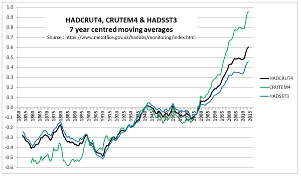
Figure 1 : Graph of Hadley Centre 7 year moving average temperature anomalies for Land (CRUTEM4), Sea (HADSST3) and Combined (HADCRUT4)
The question that needs to be answered is whether the anomalous post-1975 warming on the land is due to real divergence, or due to issues in the estimation of global average temperature anomaly.
In another post – The magnitude of Early Twentieth Century Warming relative to Post-1975 Warming – I looked at the NASA Gistemp data, which is usefully broken down into 8 Latitude Zones. A summary graph is shown in Figure 2.

Figure 2 : NASA Gistemp zonal anomalies and the global anomaly
This is more detail than the HADCRUT4 data, which is just presented as three zones of the Tropics, along with Northern and Southern Hemispheres. However, the Hadley Centre, on their HADCRUT4 Data: download page, have, under HadCRUT4 Gridded data: additional fields, a file HadCRUT.4.6.0.0.median_ascii.zip. This contains monthly anomalies for 5o by 5o grid cells from 1850 to 2017. There are 36 zones of latitude and 72 zones of longitude. Over 2016 months, there are over 5.22 million grid cells, but only 2.51 million (48%) have data. From this data, I have constructed a global temperature anomaly. The major issue in the calculation is that the grid cells are of different areas. A grid cell nearest to the equator at 0o to 5o has about 23 times the area of a grid cell adjacent to the poles at 85o to 90o. I used the appropriate weighting for each band of latitude.
The question is whether I have calculated a global anomaly similar to the Hadley Centre. Figure 3 is a reconciliation with the published global anomaly mean (available from here) and my own.
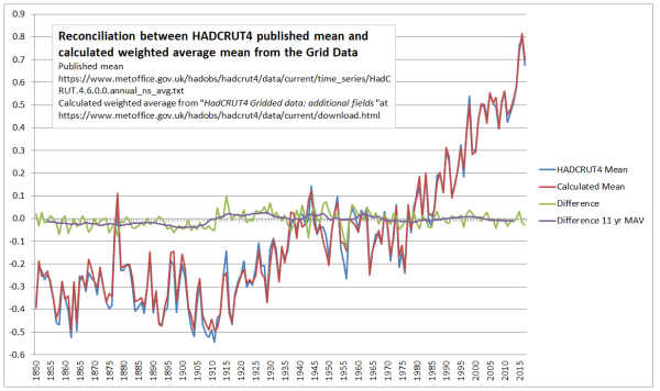
Figure 3 : Reconciliation between HADCRUT4 published mean and calculated weighted average mean from the Gridded Data
Prior to 1910, my calculations are slightly below the HADCRUT 4 published data. The biggest differences are in 1956 and 1915. Overall the differences are insignificant and do not impact on the analysis.
I split down the HADCRUT4 temperature data by eight zones of latitude on a similar basis to NASA Gistemp. Figure 4 presents the results on the same basis as Figure 2.
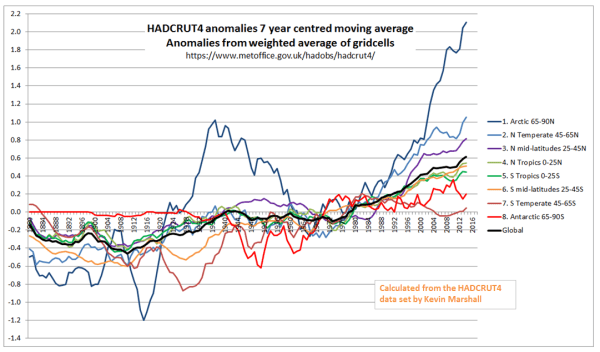
Figure 4 : Zonal surface temperature anomalies a the global anomaly calculated using the HADCRUT4 gridded data.
Visually, there are a number of differences between the Gistemp and HADCRUT4-derived zonal trends.
A potential problem with the global average calculation
The major reason for differences between HADCRUT4 & Gistemp is that the latter has infilled estimated data into areas where there is no data. Could this be a problem?
In Figure 5, I have shown the build-up in global coverage. That is the percentage of 5o by 5o grid cells with an anomaly in the monthly data.
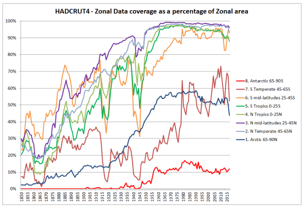
Figure 5 : HADCRUT4 Change in the percentage coverage of each zone in the HADCRUT4 gridded data.
Figure 5 shows a build-up in data coverage during the late nineteenth and early twentieth centuries. The World Wars (1914-1918 & 1939-1945) had the biggest impact on the Southern Hemisphere data collection. This is unsurprising when one considers it was mostly fought in the Northern Hemisphere, and European powers withdrew resources from their far-flung Empires to protect the mother countries. The only zones with significantly less than 90% grid coverage in the post-1975 warming period are the Arctic and the region below 45S. That is around 19% of the global area.
Finally, comparing comparable zones in the Northen and Southern hemispheres, the tropics seem to have comparable coverage, whilst for the polar, temperate and mid-latitude areas the Northern Hemisphere seems to have better coverage after 1910.
This variation in coverage can potentially lead to wide discrepancies between any calculated temperature anomalies and a theoretical anomaly based upon one with data in all the 5o by 5o grid cells. As an extreme example, with my own calculation, if just one of the 72 grid cells in a band of latitude had a figure, then an “average” would have been calculated for a band right around the world 555km (345 miles) from North to South for that month for that band. In the annual figures by zone, it only requires one of the 72 grid cells, in one of the months, in one of the bands of latitude to have data to calculate an annual anomaly. For the tropics or the polar areas, that is just one in 4320 data points to create an anomaly. This issue will impact early twentieth-century warming episode far more than the post-1975 one. Although I would expect the Hadley centre to have done some data cleanup of the more egregious examples in their calculation, potentially lack of data in grid cells could have quite random impacts, thus biasing the global temperature anomaly trends to an unknown, but significant extent. An appreciation of how this could impact can be appreciated from an example of NASA GISS Global Maps.
NASA GISS Global Maps Temperature Trends Example
NASA GISS Global Maps from GHCN v3 Data provide maps with the calculated change in average temperatures. I have run the maps to compare annual data for 1940 with a baseline of 1881-1910, capturing much of the early twentieth-century warming. The maps are at both the 1200km and 250km smoothing.

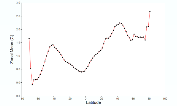
Figure 6 : NASA GISS Global anomaly Map and average anomaly by Latitude comparing 1940 with a baseline of 1881 to 1910 and a 1200km smoothing radius.
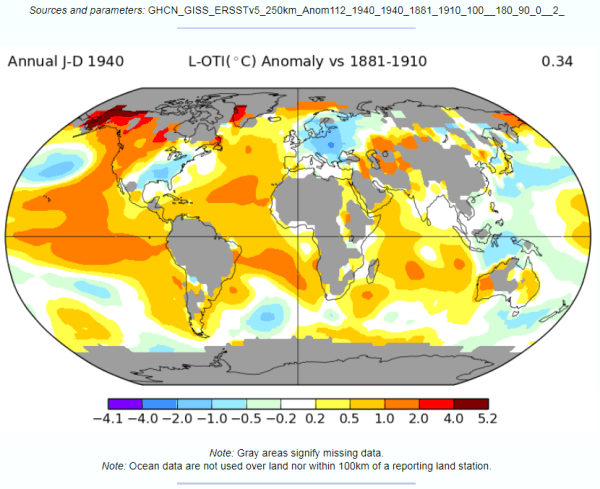
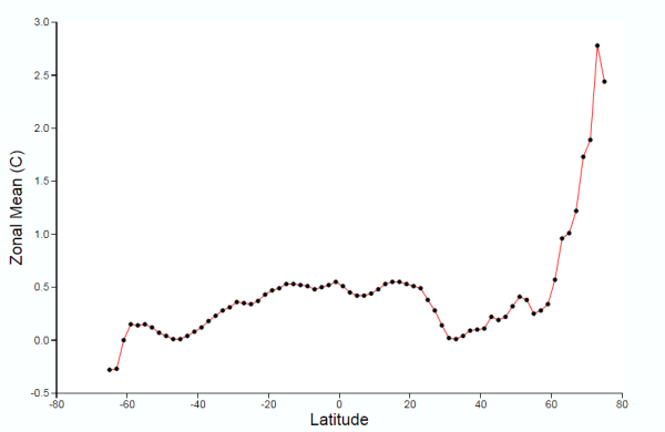
Figure 7 : NASA GISS Global anomaly Map and average anomaly by Latitude comparing 1940 with a baseline of 1881 to 1910 and a 250km smoothing radius.
With respect to the maps in figures 6 & 7
- There is no apparent difference in the sea data between the 1200km and 250km smoothing radius, except in the polar regions with more cover in the former. The differences lie in the land area.
- The grey areas with insufficient data all apply to the land or ocean areas in polar regions.
- Figure 6, with 1200km smoothing, has most of the land infilled, whilst the 250km smoothing shows the lack of data coverage for much of South America, Africa, the Middle East, South-East Asia and Greenland.
Even with these land-based differences in coverage, it is clear that from either map that at any latitude there are huge variations in calculated average temperature change. For instance, take 40N. This line of latitude is North of San Francisco on the West Coast USA, clips Philidelphia on the East Coast. On the other side of the Atlantic, Madrid, Ankara and Beijing are at about 40N. There are significant points on the line on latitude with estimate warming greater than 1C (e.g. California), whilst at the same time in Eastern Europe, cooling may have exceeded 1C in the period. More extreme is at 60N (Southern Alaska, Stockholm, St Petersburg) the difference in temperature along the line of latitude is over 3C. This compares to a calculated global rise of 0.40C.
This lack of data may have contributed (along with a faulty algorithm) to the differences in the Zonal mean charts by Latitude. The 1200km smoothing radius chart bears little relation to the 250km smoothing radius. For instance:-
- 1200km shows 1.5C warming at 45S, 250km about zero. 45S cuts through South Island, New Zealand.
- From the equator to 45N, 1200km shows rise from 0.5C to over 2.0C, 250km shows drop from less than 0.5C to near zero, then rise to 0.2C. At around 45N lies Ottowa, Maine, Bordeaux, Belgrade, Crimea and the most Northern point in Japan.
The differences in the NASA Giss Maps, in a period when available data covered only around half the 2592 5o by 5o grid cells, indicate quite huge differences in trends between different areas. As a consequence, trying to interpolate warming trends from one area to adjacent areas appears to give quite different results in terms of trends by latitude.
Conclusions and Further Questions
The issue I originally focussed upon was the relative size of the early twentieth-century warming to the Post-1975. The greater amount of warming in the later period seemed to be due to the greater warming on land covering just 30% of the total global area. The sea temperature warming phases appear to be pretty much the same.
The issue that I focussed upon was a data issue. The early twentieth century had much less data coverage than after 1975. Further, the Southern Hemisphere had worse data coverage than the Northern Hemisphere, except in the Tropics. This means that in my calculation of a global temperature anomaly from the HADCRUT4 gridded data (which in aggregate was very similar to the published HADCRUT4 anomaly) the average by latitude will not be comparing like with like in the two warming periods. In particular, in the early twentieth-century, a calculation by latitude will not average right the way around the globe, but only on a limited selection of bands of longitude. On average this was about half, but there are massive variations. This would be alright if the changes in anomalies were roughly the same over time by latitude. But an examination of NASA GISS global maps for a period covering the early twentieth-century warming phase reveals that trends in anomalies at the same latitude are quite different over time. This implies that there could be large, but unknown, biases in the data.
I do not believe the analysis ends here. There are a number of areas that I (or others) can try to explore.
- Does the NASA GISS infilling of the data get us closer or further away from a what a global temperature anomaly would look like with full data coverage? My guess, based on the extreme example of Antartica trends (discussed here) is that the infilling will move away from the more perfect trend. The data could show otherwise.
- Are the changes in data coverage on land more significant than the global average or less? Looking at CRUTEM4 data could resolve this question.
- Would anomalies based upon similar grid coverage after 1900 give different relative trend patterns to the published ones based on dissimilar grid coverage?
Whether I get the time to analyze these is another issue.
Finally, the problem of trends varying considerably and quite randomly across the globe is the same issue that I found with land data homogenisation discussed here and here. To derive a temperature anomaly for a grid cell, it is necessary to make the data homogeneous. In standard homogenisation techniques, it is assumed that the underlying trends in an area is pretty much the same. Therefore, any differences in trend between adjacent temperature stations will be as a result of data imperfections. I found numerous examples where there were likely differences in trend between adjacent temperature stations. Homogenisation will, therefore, eliminate real but local climatic trends. Averaging incomplete global data where missing data could contain regional but unknown data trends may cause biases at a global scale.